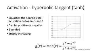
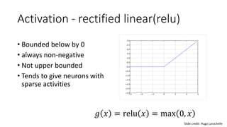
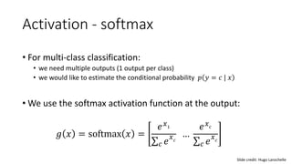
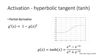
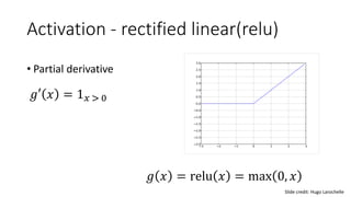
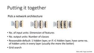
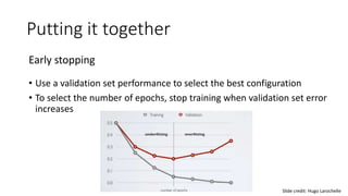
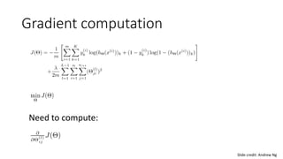
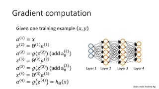
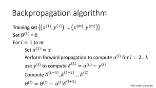
This document provides an overview of neural networks, including: - The origins and basic structure of artificial neurons and neural networks with multiple layers. - Common activation functions like sigmoid, tanh, ReLU, and softmax. - The universal approximation theorem which states neural networks can approximate continuous functions. - How neural networks perform forward and backward propagation to compute gradients and update weights during training. Techniques like initialization, early stopping, and dropout help optimize training.

1. Neural Networks II
Chen Gao
Virginia Tech Spring 2019
ECE-5424G / CS-5824

2. Neural Networks
• Origins: Algorithms that try to mimic the brain.
What is this?

3. A single neuron in the brain
Input
Output Slide credit: Andrew Ng

4. An artificial neuron: Logistic unit
𝑥 =
𝑥0
𝑥1
𝑥2
𝑥3
𝜃 =
𝜃0
𝜃1
𝜃2
𝜃3
• Sigmoid (logistic) activation function
𝑥1
𝑥2
𝑥3
𝑥0
ℎ𝜃 𝑥 =
1
1 + 𝑒−𝜃⊤𝑥
“Bias unit”
“Input”
“Output”
“Weights”
“Parameters”
Slide credit: Andrew Ng

5. Visualization of weights, bias, activation function
bias b only change the
position of the hyperplane
Slide credit: Hugo Larochelle
range
determined
by g(.)

6. Activation - sigmoid
• Squashes the neuron’s pre-
activation between 0 and 1
• Always positive
• Bounded
• Strictly increasing
𝑔 𝑥 =
1
1 + 𝑒−𝑥
Slide credit: Hugo Larochelle

7. Activation - hyperbolic tangent (tanh)
• Squashes the neuron’s pre-
activation between -1 and 1
• Can be positive or negative
• Bounded
• Strictly increasing
𝑔 𝑥 = tanh 𝑥 =
𝑒𝑥
− 𝑒−𝑥
𝑒𝑥 + 𝑒−𝑥
Slide credit: Hugo Larochelle

8. Activation - rectified linear(relu)
• Bounded below by 0
• always non-negative
• Not upper bounded
• Tends to give neurons with
sparse activities
Slide credit: Hugo Larochelle
𝑔 𝑥 = relu 𝑥 = max 0, 𝑥

9. Activation - softmax
• For multi-class classification:
• we need multiple outputs (1 output per class)
• we would like to estimate the conditional probability 𝑝 𝑦 = 𝑐 | 𝑥
• We use the softmax activation function at the output:
𝑔 𝑥 = softmax 𝑥 =
𝑒𝑥1
𝑐 𝑒
𝑥𝑐
…
𝑒𝑥𝑐
𝑐 𝑒
𝑥𝑐
Slide credit: Hugo Larochelle

10. Universal approximation theorem
‘‘a single hidden layer neural network with a linear output unit
can approximate any continuous function arbitrarily well,
given enough hidden units’’
Hornik, 1991
Slide credit: Hugo Larochelle

11. Neural network – Multilayer
𝑎1
(2)
𝑎2
(2)
𝑎3
(2)
𝑎0
(2)
ℎΘ 𝑥
Layer 1
“Output”
𝑥1
𝑥2
𝑥3
𝑥0
Layer 2 (hidden) Layer 3 Slide credit: Andrew Ng

12. Neural network
𝑎1
(2)
𝑎2
(2)
𝑎3
(2)
𝑎0
(2)
ℎΘ 𝑥
𝑥1
𝑥2
𝑥3
𝑥0
𝑎𝑖
(𝑗)
= “activation” of unit 𝑖 in layer 𝑗
Θ 𝑗 = matrix of weights controlling
function mapping from layer 𝑗 to layer 𝑗 + 1
𝑎1
(2)
= 𝑔 Θ10
(1)
𝑥0 + Θ11
(1)
𝑥1 + Θ12
(1)
𝑥2 + Θ13
(1)
𝑥3
𝑎2
(2)
= 𝑔 Θ20
(1)
𝑥0 + Θ21
(1)
𝑥1 + Θ22
(1)
𝑥2 + Θ23
(1)
𝑥3
𝑎3
(2)
= 𝑔 Θ30
(1)
𝑥0 + Θ31
(1)
𝑥1 + Θ32
(1)
𝑥2 + Θ33
(1)
𝑥3
ℎΘ(𝑥) = 𝑔 Θ10
(2)
𝑎0
(2)
+ Θ11
(1)
𝑎1
(2)
+ Θ12
(1)
𝑎2
(2)
+ Θ13
(1)
𝑎3
(2)
𝑠𝑗 unit in layer 𝑗
𝑠𝑗+1 units in layer 𝑗 + 1
Size of Θ 𝑗
?
𝑠𝑗+1 × (𝑠𝑗 + 1)
Slide credit: Andrew Ng

13. Neural network
𝑎1
(2)
𝑎2
(2)
𝑎3
(2)
𝑎0
(2)
ℎΘ 𝑥
𝑥1
𝑥2
𝑥3
𝑥0
𝑥 =
𝑥0
𝑥1
𝑥2
𝑥3
z(2) =
z1
(2)
z2
(2)
z3
(2)
𝑎1
(2)
= 𝑔 Θ10
(1)
𝑥0 + Θ11
(1)
𝑥1 + Θ12
(1)
𝑥2 + Θ13
(1)
𝑥3 = 𝑔(z1
(2)
)
𝑎2
(2)
= 𝑔 Θ20
(1)
𝑥0 + Θ21
(1)
𝑥1 + Θ22
(1)
𝑥2 + Θ23
(1)
𝑥3 = 𝑔(z2
(2)
)
𝑎3
(2)
= 𝑔 Θ30
(1)
𝑥0 + Θ31
(1)
𝑥1 + Θ32
(1)
𝑥2 + Θ33
(1)
𝑥3 = 𝑔(z3
(2)
)
ℎΘ 𝑥 = 𝑔 Θ10
2
𝑎0
2
+ Θ11
1
𝑎1
2
+ Θ12
1
𝑎2
2
+ Θ13
1
𝑎3
2
= 𝑔(𝑧(3))
“Pre-activation”
Slide credit: Andrew Ng
Why do we need g(.)?

14. Neural network
𝑎1
(2)
𝑎2
(2)
𝑎3
(2)
𝑎0
(2)
ℎΘ 𝑥
𝑥1
𝑥2
𝑥3
𝑥0
𝑥 =
𝑥0
𝑥1
𝑥2
𝑥3
z(2) =
z1
(2)
z2
(2)
z3
(2)
𝑎1
(2)
= 𝑔(z1
(2)
)
𝑎2
(2)
= 𝑔(z2
(2)
)
𝑎3
(2)
= 𝑔(z3
(2)
)
ℎΘ 𝑥 = 𝑔(𝑧(3)
)
“Pre-activation”
𝑧(2)
= Θ(1)
𝑥 = Θ(1)
𝑎(1)
𝑎(2)
= 𝑔(𝑧(2)
)
Add 𝑎0
(2)
= 1
𝑧(3)
= Θ(2)
𝑎(2)
ℎΘ 𝑥 = 𝑎(3)
= 𝑔(𝑧(3)
)
Slide credit: Andrew Ng

15. Flow graph - Forward propagation
𝑎
(2)
𝑧
(2)
𝑎
(3)
ℎΘ 𝑥
X
𝑊
(1)
𝑏
(1)
𝑧
(3)
𝑊
(2)
𝑏
(2)
𝑧(2)
= Θ(1)
𝑥 = Θ(1)
𝑎(1)
𝑎(2)
= 𝑔(𝑧(2)
)
Add 𝑎0
(2)
= 1
𝑧(3)
= Θ(2)
𝑎(2)
ℎΘ 𝑥 = 𝑎(3)
= 𝑔(𝑧(3)
)
How do we evaluate
our prediction?

16. Cost function
Logistic regression:
Neural network:
Slide credit: Andrew Ng

17. Gradient computation
Need to compute:
Slide credit: Andrew Ng

18. Gradient computation
Given one training example 𝑥, 𝑦
𝑎(1)
= 𝑥
𝑧(2)
= Θ(1)
𝑎(1)
𝑎(2)
= 𝑔(𝑧(2)
) (add a0
(2)
)
𝑧(3)
= Θ(2)
𝑎(2)
𝑎(3)
= 𝑔(𝑧(3)
) (add a0
(3)
)
𝑧(4)
= Θ(3)
𝑎(3)
𝑎(4)
= 𝑔 𝑧 4
= ℎΘ 𝑥
Slide credit: Andrew Ng

19. Gradient computation: Backpropagation
Intuition: ߜ𝑗
(𝑙)
= “error” of node 𝑗 in layer 𝑙
For each output unit (layer L = 4)
Slide credit: Andrew Ng
ߜ(4) = 𝑎(4) − 𝑦
ߜ(3) = ߜ(4) 𝜕ߜ(4)
𝜕𝑧(3) = ߜ(4) 𝜕ߜ(4)
𝜕𝑎(4)
𝜕𝑎(4)
𝜕𝑧(4)
𝜕𝑧(4)
𝜕𝑎(3)
𝜕𝑎(3)
𝜕𝑧(3)
= 1 *Θ 3 𝑇
ߜ(4)
.∗ 𝑔′ 𝑧 4
.∗ 𝑔′(𝑧(3)
)
𝑧(3)
= Θ(2)
𝑎(2)
𝑎(3)
= 𝑔(𝑧(3)
)
𝑧(4)
= Θ(3)
𝑎(3)
𝑎(4)
= 𝑔 𝑧 4

20. Backpropagation algorithm
Training set 𝑥(1)
, 𝑦(1)
… 𝑥(𝑚)
, 𝑦(𝑚)
Set Θ(1)
= 0
For 𝑖 = 1 to 𝑚
Set 𝑎(1)
= 𝑥
Perform forward propagation to compute 𝑎(𝑙)
for 𝑙 = 2. . 𝐿
use 𝑦(𝑖)
to compute ߜ
(𝐿)
= 𝑎(𝐿)
− 𝑦(𝑖)
Compute ߜ
(𝐿−1)
, ߜ
(𝐿−2)
… ߜ
(2)
Θ(𝑙)
= Θ(𝑙)
− 𝑎(𝑙)
ߜ
(𝑙+1)
Slide credit: Andrew Ng

21. Activation - sigmoid
• Partial derivative
𝑔 𝑥 =
1
1 + 𝑒−𝑥
Slide credit: Hugo Larochelle
𝑔′ 𝑥 = 𝑔 𝑥 1 − 𝑔 𝑥

22. Activation - hyperbolic tangent (tanh)
𝑔 𝑥 = tanh 𝑥 =
𝑒𝑥
− 𝑒−𝑥
𝑒𝑥 + 𝑒−𝑥
Slide credit: Hugo Larochelle
• Partial derivative
𝑔′ 𝑥 = 1 − 𝑔 𝑥 2

23. Activation - rectified linear(relu)
Slide credit: Hugo Larochelle
𝑔 𝑥 = relu 𝑥 = max 0, 𝑥
• Partial derivative
𝑔′ 𝑥 = 1𝑥 > 0

24. Initialization
• For bias
• Initialize all to 0
• For weights
• Can’t initialize all weights to the same value
• we can show that all hidden units in a layer will always behave the same
• need to break symmetry
• Recipe: U[-b, b]
• the idea is to sample around 0 but break symmetry
Slide credit: Hugo Larochelle

25. Putting it together
Pick a network architecture
Slide credit: Hugo Larochelle
• No. of input units: Dimension of features
• No. output units: Number of classes
• Reasonable default: 1 hidden layer, or if >1 hidden layer, have same no.
of hidden units in every layer (usually the more the better)
• Grid search

26. Putting it together
Early stopping
Slide credit: Hugo Larochelle
• Use a validation set performance to select the best configuration
• To select the number of epochs, stop training when validation set error
increases

27. Other tricks of the trade
Slide credit: Hugo Larochelle
• Normalizing your (real-valued) data
• Decaying the learning rate
• as we get closer to the optimum, makes sense to take smaller update steps
• mini-batch
• can give a more accurate estimate of the risk gradient
• Momentum
• can use an exponential average of previous gradients

28. Dropout
Slide credit: Hugo Larochelle
• Idea: «cripple» neural network by removing hidden units
• each hidden unit is set to 0 with probability 0.5
• hidden units cannot co-adapt to other units
• hidden units must be more generally useful