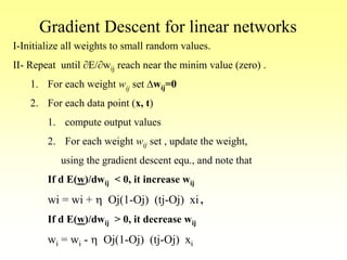
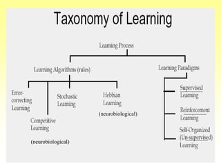
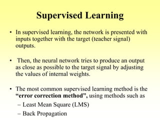
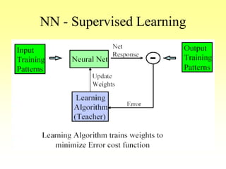
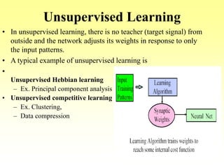
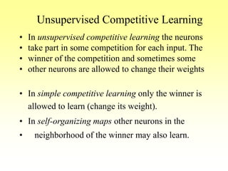
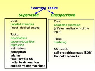
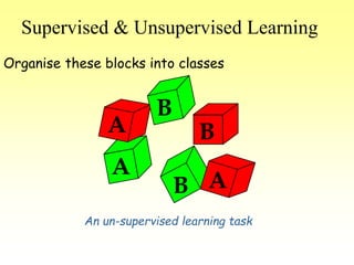
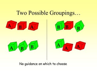
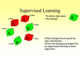
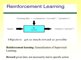
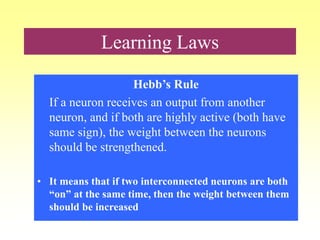
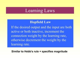
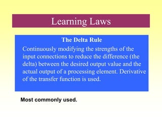
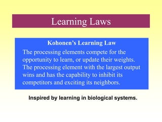
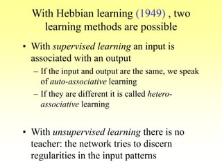
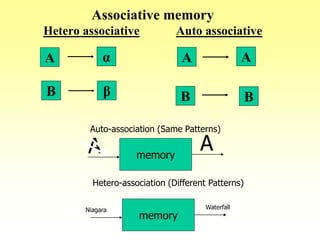
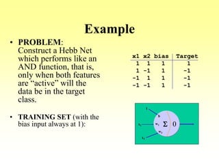
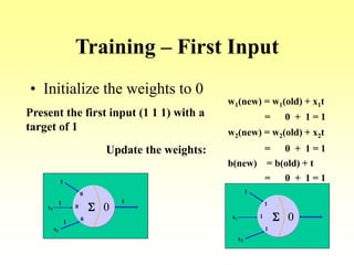
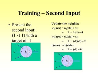
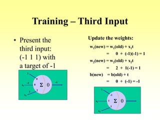
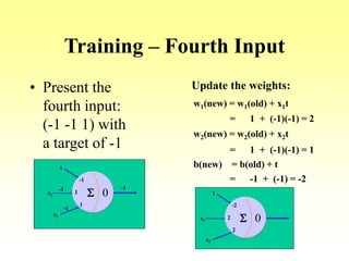
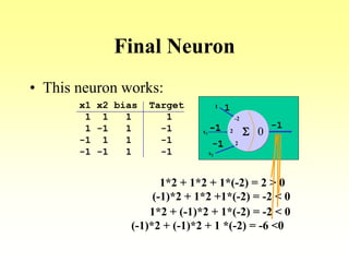
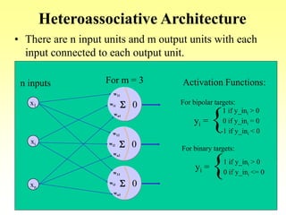
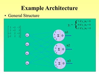
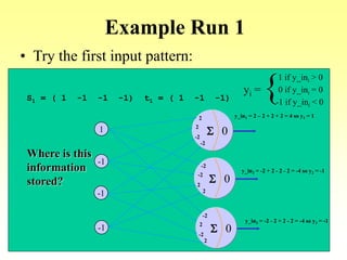
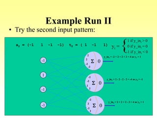
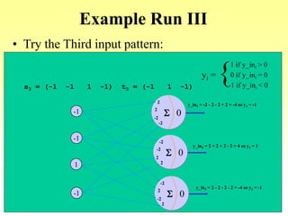
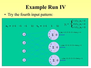
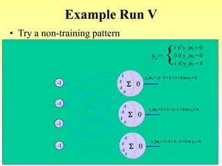
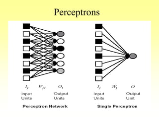
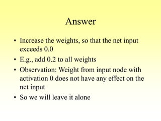
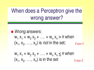
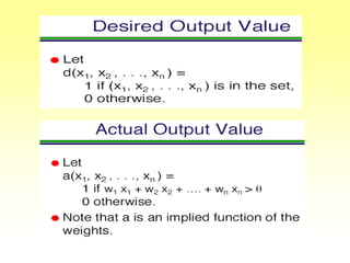
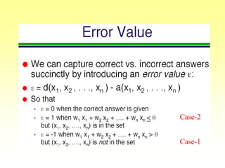
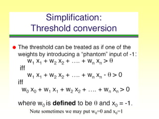
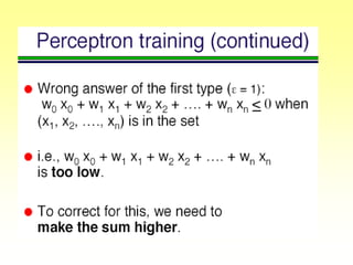
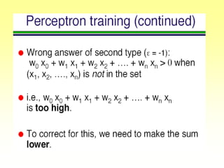
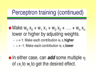
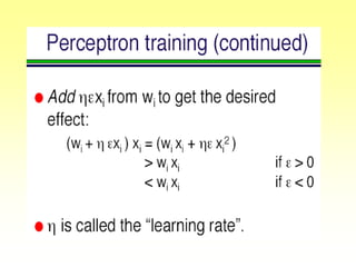
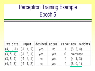
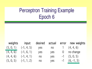
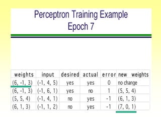
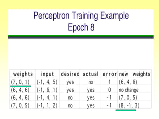
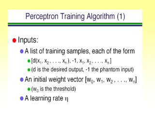
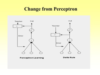
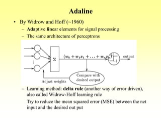
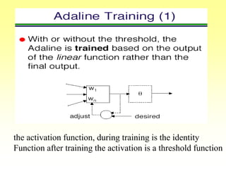
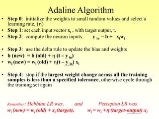
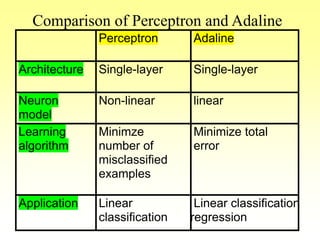
This document discusses various learning processes and techniques used in neural networks. It describes supervised learning where a network is presented inputs and target outputs to learn from, and unsupervised learning where there is no external target and the network learns from the inputs alone. Specific unsupervised techniques mentioned are Hebbian learning, competitive learning, and self-organizing maps. Supervised learning algorithms covered include least mean square and backpropagation. The document also provides examples of Hebbian learning for associative memory using hetero-associative networks.


![Alternative View
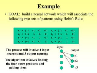
• Goal: Associate an input vector with a specific output
vector in a neural net
• In this case, Hebb’s Rule is the same as taking the outer
product of the two vectors:
s = (s1, . . ., si, . . . sn) and t = (t1, . . ., ti, . . . tm)
st = [t1 … tm] =
s1
sn
.
.
.
s1t1 s1tm
snt1 sntm
.
.
.
. . Weight matrix](https://image.slidesharecdn.com/lec-3-4-5-learning-200207114421/85/Lec-3-4-5-learning-31-320.jpg)
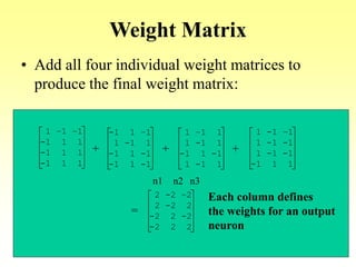
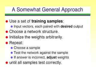
![Weight Matrix
• To store more than one association in a neural net
using Hebb’s Rule
– Add the individual weight matrices
• This method works only if the input vectors for each
association are orthogonal (uncorrelated)
– That is, if their dot product is 0
s = (s1, . . ., si, . . . sn) and t = (t1, . . ., ti, . . . tm)
s t = [s1 … sn]
t1
tm
.
.
.
= 0](https://image.slidesharecdn.com/lec-3-4-5-learning-200207114421/85/Lec-3-4-5-learning-32-320.jpg)

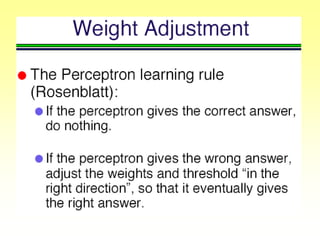
![Algorithm
1
-1
-1
-1
[ 1 –1 –1] =
1 –1 –1
-1 1 1
-1 1 1
-1 1 1
Pattern pair 1:
-1
1
-1
-1
[ 1 –1 1] =
-1 1 –1
1 -1 1
-1 1 -1
-1 1 -1
Pattern pair 2:
-1
-1
1
-1
[-1 1 –1] =
1 –1 1
1 -1 1
-1 1 -1
1 -1 1
Pattern pair 3:
-1
-1
-1
1
[-1 1 1] =
1 -1 –1
1 -1 -1
1 -1 -1
-1 1 1
Pattern pair 4:](https://image.slidesharecdn.com/lec-3-4-5-learning-200207114421/85/Lec-3-4-5-learning-36-320.jpg)
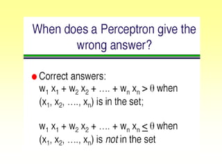
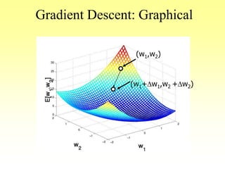
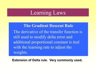
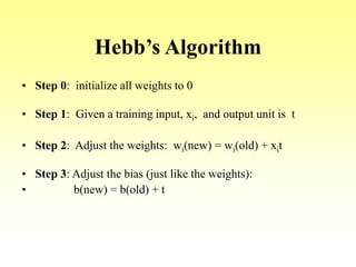
![Gradient Descent Learning Rule
• Consider linear unit without threshold and
continuous output o (not just –1,1)
o= -w0 + w1 x1 + … + wn xn
• Train the wi’s such that they minimize the squared
error
– E[w1,…,wn] = ½ SjD (tj-oj)2
where D is the set of training examples](https://image.slidesharecdn.com/lec-3-4-5-learning-200207114421/85/Lec-3-4-5-learning-106-320.jpg)
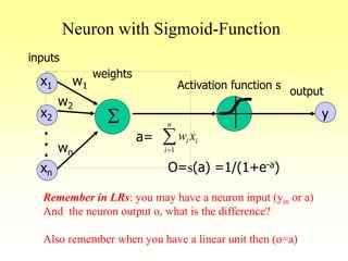
![Sigmoid Unit
S
x1
x2
xn
.
.
.
w1
w2
wn
w0
x0=-1
a=
O
O=s(a)=1/(1+e-a)
Note that :
If s(x) is the sigmoid function: 1/(1+e-x)
then ds(x)/dx= s(x) (1- s(x)), proof that.
Derive gradient decent rules to train:one sigmoid function
Dw = E/wi = h O (1-O) (tj-O) xi (try to proof that)
n
i
ii xw
1
Scince, E[w1,…,wn] = ½ SjD (tj-oj)2](https://image.slidesharecdn.com/lec-3-4-5-learning-200207114421/85/Lec-3-4-5-learning-108-320.jpg)
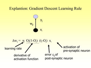
![Gradient Descent Rule
• Gradient descent rule, update the the weight
value using the equation:
wi = wi + h Oj(1-Oj) (tj-Oj) xi
derived from minimization of error function
E[w1,…,wn] = ½ Sj (t-y)2
by means of gradient descent.](https://image.slidesharecdn.com/lec-3-4-5-learning-200207114421/85/Lec-3-4-5-learning-111-320.jpg)