Mathematics behind Machine Learning: Linear Regression Model

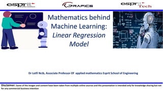
1. Mathematics behind
Machine Learning:
Linear Regression
Model
Dr Lotfi Ncib, Associate Professor Of applied mathematics Esprit School of Engineering
Disclaimer: Some of the Images and content have been taken from multiple online sources and this presentation is intended only for knowledge sharing but not
for any commercial business intention

2. 1
What is The difference between AI, ML and DL?
• Artificial Intelligence AI tries to make computers intelligent in order to mimic
the cognitive functions of humans. So, AI is a general field with a broad scope
including:
• Computer Vision,
• Language Processing,
• Creativity…
• Machine Learning ML is the branch of AI that covers the statistical part of
artificial intelligence. It teaches the computer to solve problems by looking at
hundreds or thousands of examples, learning from them, and then using that
experience to solve the same problem in new situations:
• Regression,
• Classification,
• Clustering…
• DL is a very special field of Machine Learning where computers can actually
learn and make intelligent decisions on their own,
• CNN
• RNN…

3. 2
Types of Machine Learning

4. 3
Classical Machine Learning
F

5. 4
What is Regression?
Size (feet2) Number of
bedrooms
Number of
floors
Age of home
(years) Price ($1000)
2104 5 1 45 460
1416 3 2 40 232
1534 3 2 30 315
852 2 1 36 178
1510 3 2 30 ?
Regression is the
process of predicting
a continuous value.
X: Independent variable Y: dependent variable
Continuousvariable
Regression is Supervised: Target is provided

6. 5
Types of Regression
• Simple Regression
• Simple Linear Regression
• Simple Non-Linear Regression.
Predict Price($1000) vs Size(feet2) of all houses
• Multiple Regression
• Multiple Linear Regression
• Multiple Non-Linear Regression.
Predict Price($1000) vs Size(feet2) and number of
bedrooms
Types of Regression
Simple
Linear Non-Linear
Multiple
Linear Non-Linear
One Variable 2+ Variables

7. 6
Applications of Regression
• Price estimation of house:
• size, number of bedrooms, and so on.
• Employment income:
• hours of work, education, occupation, sex age, years of
experience, and so on.
Indeed you can find many examples of the usefulness of regression
analysis in these and many other fields, or domains such as finance,
healthcare, retail, and more.

8. 7
Exemple of Regression algorithms
We have many regression algorithms:
• Ordinal regression
• Poisson regression
• Fast forest quantile regression
• Linear, polynomial, Lasso, Stepwise, Ridge regression
• Bayesian linear regression
• Neural network regression
• Decision forest regression
• KNN
• Boosted decision tree regression

9. 8
Simple Linear
regression
Model
representation

10. 9
Simple Linear Regression
• Simple linear regression
• Predict Price($1000) vs Size(feet2) of all houses
• Independent variable (x): Size of house
• Dependent variable (y): Price of house
Size in feet2 (x) Price ($) in 1000 (y)
2104 460
1416 232
1534 315
852 178
1245 ?
Notation:
m = Number of training examples
x = “input” variable / features
y = “output” variable / “target” variable

11. 10
Training Set
Learning Algorithm
h
Size of
house
Estimated
price
hypothesis Linear regression with one variable.
Univariate linear regression.
Model representation
ℎ 𝜃 𝑥 = 𝜃0 + 𝜃1 𝑥
Choice of ℎ ?

12. 11
Cost function
Training Set Size in feet2 (x) Price ($) in 1000 (y)
2104 460
1416 232
1534 315
852 178
Goal: Find regression line that makes
sum of residuals as small as possible
ℎ 𝜃 𝑥 = 𝜃0 + 𝜃1 𝑥
Hypothesis :
𝜃0, 𝜃1Parameters :

13. 12
Cost function
Idea: Choose 𝜃0, 𝜃1 so that ℎ 𝜃 is close to 𝑦 for our training samples
𝐽 𝜃0, 𝜃1 =
1
2𝑚
෍
𝑖=1
𝑚
(ℎ 𝜃(𝑥 𝑖 ) − 𝑦 𝑖 )2
𝜃0, 𝜃1
ℎ 𝜃 𝑥 = 𝜃0 + 𝜃1 𝑥Hypothesis :
Parameters :
Cost function :
min
𝜃0,𝜃1
𝐽 𝜃0, 𝜃1Goal :

14. 13
Analytical Solution
the vectorization expression of linear regression cost function can be denoted as:
𝑋 =
1 𝑥(1)
⋮ ⋮
1 𝑥(𝑚)
𝜃 =
𝜃0
𝜃1
𝐽 𝜃 =
1
2𝑚
𝑋𝜃 − 𝑦 𝑇
(𝑋𝜃 − 𝑦)
𝐽 𝜃 = 𝑋𝜃 − 𝑦 𝑇(𝑋𝜃 − 𝑦)
𝐽 𝜃 = ( 𝑋𝜃 𝑇
− 𝑦 𝑇
)(𝑋𝜃 − 𝑦)
Since
1
2𝑚
is a constant, we omit this constant term. Then our cost function becomes:
𝑦 =
𝑦(1)
⋮
𝑦(𝑚)
This can be further simplified as:
We expand it to obtain: 𝐽 𝜃 = 𝑋𝜃 𝑇 𝑋𝜃 − 𝑋𝜃 𝑇 𝑦 − 𝑦 𝑇 𝑋𝜃 + 𝑦 𝑇 𝑦
Cost function: 𝐽 𝜃0, 𝜃1 =
1
2𝑚
෍
𝑖=1
𝑚
(ℎ 𝜃(𝑥 𝑖
) − 𝑦 𝑖
)2
Or ( 𝑋𝜃 𝑇
𝑦) 𝑇
= 𝑦 𝑇
(𝑋𝜃) Then 𝐽 𝜃 = 𝑋𝜃 𝑇 𝑋𝜃 − 2𝑦 𝑇 𝑋𝜃 + 𝑦 𝑇 𝑦

15. 14
Further more, we can write it as: 𝐽 𝜃 = 𝜃 𝑇
𝑋 𝑇
𝑋𝜃 − 2𝑦 𝑇
𝑋𝜃 + 𝑦 𝑇
𝑦
Now we need to take derivative of the cost function. For convenience, the common matrix derivative
formulas are listed as reference:
𝜕𝐴𝑋
𝜕𝑋
= 𝐴,
𝜕𝑋 𝑇 𝐴
𝜕𝑋
= 𝐴,
𝜕𝑋 𝑇 𝑋
𝜕𝑋
= 2𝑋,
𝜕𝑋 𝑇 𝐴𝑋
𝜕𝑋
= 𝐴𝑋 + 𝐴 𝑇 𝑋
Using the above formulas, we can derive our cost function respect to 𝜃 as:
𝜕𝐽 𝜃
𝜕𝜃
= 2𝑋 𝑇
𝑋𝜃 − 2𝑋 𝑇
𝑦
In order to solve the variables, we need to make the above derivation equal to zero, that is:
2𝑋 𝑇
𝑋𝜃 − 2𝑋 𝑇
𝑦 = 0 then 𝑋 𝑇
𝑋𝜃 = 𝑋 𝑇
𝑦
Thus we can compute θ as: 𝜃 = (𝑋 𝑇
𝑋)−1
𝑋 𝑇
𝑦
Analytical Solution
- What if 𝑋 𝑇 𝑋 is non-invertible? (singular/ degenerate)

16. 15
Gradient descent
Have some function
Want
Outline:
• Start with some
• Keep changing to reduce
until we hopefully end up at a minimum

17. 16
Gradient descent algorithm
Correct: Simultaneous update Incorrect:
Gradient descent

18. 17
Gradient descent
Gradient descent algorithm Linear Regression Model
update
and
simultaneously

19. 18
Multiple Linear
regression
Model
representation

20. 19
Size (feet2) Number of
bedrooms
Number of
floors
Age of home
(years) Price ($1000)
2104 5 1 45 460
1416 3 2 40 232
1534 3 2 30 315
852 2 1 36 178
1510 3 2 30 ?
Notation:
m = Number of training examples
n = Number of features(variables)
𝑥(𝑖)
= “input” of the 𝑖 𝑡ℎ
training example
𝑥𝑗
(𝑖)
= value of feature 𝑗 in 𝑖 𝑡ℎ training example
Model representation

21. 20
Training Set
Learning Algorithm
h
Size of house,
Number of bedrooms,
Numbers of floors,
Age of home
Estimated
price
hypothesis
Choice of h ?
Model representation
ℎ 𝜃 𝑥 = 𝜃0 + 𝜃1 𝑥
ℎ 𝜃 𝑥 = 𝜃0 + 𝜃1 𝑥1 + 𝜃2 𝑥2 + 𝜃3 𝑥3 + 𝜃4 𝑥4

22. 21
Model representation
ℎ 𝜃 𝑥(𝑖)
= 𝜃0 + 𝜃1 𝑥1
(𝑖)
+ 𝜃2 𝑥2
(𝑖)
+ 𝜃3 𝑥3
(𝑖)
+ 𝜃4 𝑥4
(𝑖)
For convenience of notation, define 𝑥0
(𝑖)
= 1
𝑥(𝑖) =
𝑥0
(𝑖)
𝑥1
(𝑖)
𝑥2
(𝑖)
⋮
𝑥 𝑛
(𝑖)
𝜖ℝ 𝑛+1, 𝜃 =
𝜃0
𝜃1
𝜃2
⋮
𝜃 𝑛
𝜖ℝ 𝑛+1
Multivariate Linear regression
Hypothesis :
= 𝜃 𝑇
𝑥(𝑖)
ℎ 𝜃 𝑥(𝑖) = 𝜃0 + 𝜃1 𝑥1
(𝑖)
+ 𝜃2 𝑥2
(𝑖)
+ 𝜃3 𝑥3
(𝑖)
+ 𝜃4 𝑥4
(𝑖)

23. 22
Cost function
Idea: Choose 𝜃0, 𝜃1,… 𝜃 𝑛 so that ℎ 𝜃 is close to 𝑦 for our training samples
𝐽 𝜃0, 𝜃1,… 𝜃 𝑛 =
1
2𝑚
෍
𝑖=1
𝑚
(ℎ 𝜃(𝑥 𝑖
) − 𝑦 𝑖
)2
𝜃0, 𝜃1,… 𝜃 𝑛
Hypothesis :
Parameters :
Cost function :
min
𝜃0,𝜃1,… 𝜃 𝑛
𝐽 𝜃0, 𝜃1,… 𝜃 𝑛Goal :
ℎ 𝜃 𝑥(𝑖) = 𝜃0 + 𝜃1 𝑥1
(𝑖)
+ 𝜃2 𝑥2
(𝑖)
+ 𝜃3 𝑥3
(𝑖)
+ 𝜃4 𝑥4
(𝑖)
In order to achieve the hypothesis for all the samples we use the following equation:
ℎ 𝜃 𝑥 = 𝑋𝜃 =
𝑥0
(1)
𝑥1
(1)
… 𝑥 𝑛
(1)
𝑥0
(2)
⋮
𝑥1
(2)
⋮
…
…
𝑥 𝑛
(2)
⋮
𝑥0
(𝑚)
𝑥1
(𝑚)
… 𝑥 𝑛
(𝑚)
𝜃0
𝜃1
⋮
𝜃 𝑛

24. 23
Analytical Solution
the vectorization expression of linear regression cost function can be denoted as:
𝑋 =
𝑥0
(1)
𝑥1
(1)
… 𝑥 𝑛
(1)
𝑥0
(2)
⋮
𝑥1
(2)
⋮
…
…
𝑥 𝑛
(2)
⋮
𝑥0
(𝑚)
𝑥1
(𝑚)
… 𝑥 𝑛
(𝑚)
𝜃 =
𝜃0
𝜃1
⋮
𝜃 𝑛
𝐽 𝜃 =
1
2𝑚
𝑋𝜃 − 𝑦 𝑇(𝑋𝜃 − 𝑦)
𝑦 =
𝑦(1)
𝑦(2)
⋮
𝑦(𝑚)
Cost function: 𝐽 𝜃0, 𝜃1,… 𝜃 𝑛 =
1
2𝑚
෍
𝑖=1
𝑚
(ℎ 𝜃(𝑥 𝑖 ) − 𝑦 𝑖 )2
Thus we can compute 𝜃 as: 𝜃 = (𝑋 𝑇 𝑋)−1 𝑋 𝑇 𝑦
- What if 𝑋 𝑇 𝑋 is non-invertible? (singular/ degenerate)

25. 24
Gradient Descent
Repeat
Previously (n=1):
New algorithm :
Repeat
Gradient descent

26. 25
E.g. 𝑥1= size (0-2000 feet2)
𝑥2 = number of bedrooms (1-5)
Feature Scaling
Idea: Make sure features are on a similar scale.
Replace 𝑥𝑖 with 𝑥𝑖 − 𝜇𝑖 to make features have approximately zero mean
(Do not apply to 𝑥0 = 1 ).
Mean normalization
E.g.
Gradient descent in practice : Feature Scaling

27. 26
Gradient descent in practice : Feature Scaling
Gradient descent
- “Debugging”: How to make sure gradient
descent is working correctly.
- How to choose learning rate .
- If is too small: slow convergence.
- If is too large: may not decrease on
every iteration; may not converge.
To choose , try
Summary: