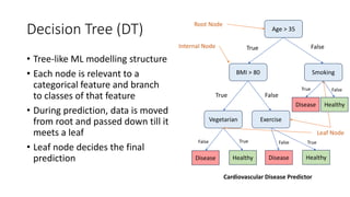
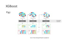
Decision Trees and Ensemble Methods is a different form of Machine Learning algorithm classes. This was one of the lectures of a full course I taught in University of Moratuwa, Sri Lanka on 2023 second half of the year.

1. DA 5230 – Statistical & Machine Learning
Lecture 9 – Decision Trees and Ensemble
Methods
Maninda Edirisooriya
manindaw@uom.lk

2. Decision Tree (DT)
• Tree-like ML modelling structure
• Each node is relevant to a
categorical feature and branch
to classes of that feature
• During prediction, data is moved
from root and passed down till it
meets a leaf
• Leaf node decides the final
prediction
BMI > 80
Age > 35
Smoking
Vegetarian Exercise
True False
True False
Cardiovascular Disease Predictor
Root Node
Internal Node
Leaf Node
Disease Healthy Disease Healthy
Disease Healthy
True
False True
False
True False

3. Decision Trees
• Suppose you have got a binary classification problem with 3
independent binary categorical variables X1, X2, X3, and 1 dependent
variable Y
• You can draw a decision tree starting from one of the X variables
• If this X variable cannot classify the training dataset perfectly, add
another X variable as a child node to the tree branches where there
are misclassifications (or not Pure)
• Even after adding the second X variable, if there are some
misclassifications in the branches, you can add the third X variable as
well OR you can add the third variable as the second node of the root

4. Decision Trees
You will be able to draw several trees like that, depending on the
training set and the X variables (note that outputs are not shown here)
Depth
1
Root X1
X2 X3
Depth
1
Root X1
X2 Depth
2
Depth
1
Root X1
X2
X3
Root
X1

5. Optimizing Decision Trees
• In order to find the maximum Purity of the classification you will have
to try with many decision trees
• As the number of parameters (nodes and their classes) are different
in each of the decision tree, there is no optimization algorithm to
minimize the error (or impurity)
• Known algorithms to find the globally optimum Decision Tree are
computationally expensive (problem known as a NP-hard Problem)
• Therefore, heuristic techniques are used to get better performance
out of Decision Trees

6. CART Algorithm
• CART (Classification And Regression Tree) is one of the best heuristic
Decision Tree algorithms
• There are 2 key decisions to be taken in the CART algorithm
1. How to select the X variable to be selected to split on each node?
2. What is the stopping criteria of splitting?
• Decision 1 is taken based on the basis of maximizing the Purity of
classification on the selected node
• Decision 2 is taken based on the basis either on,
• Reduction of purity added with new nodes
• Increased computational/memory complexity of new nodes

7. Stopping Criteria of Splitting
Splitting to a new node (being a leaf node) can be stopped with one of
the following criteria
• When all the data in the current node belongs to a one Y class
• Adding a new node exceeds the maximum depth of the tree
• Impurity reduction is less than a pre-defined threshold
• Number of data in the current node is lesser than a pre-defined
threshold

8. Adding a New Node (Splitting)
• A new node is added to a tree node, only when that branch has data
belongs to more than a one Y class (i.e. when impurity is there)
• When a new node is added, the total impurity of the new node
branches should be lesser than the current node
• Therefore, the new node is selected which has the capability of
increasing the purity (or reducing the impurity) as much as possible
• There are mainly 2 measurements to evaluate the impurity reduction,
1. Gini Index
2. Entropy
3. Variance (in Regression Trees)

9. Gini Index
• Gini Index (or Gini Impurity) is a well-known measure to evaluate the
value of discrimination between classes based on frequency
• Gini Impurity is defined as,
Gini Impurity = 1 - ෌𝐢=𝟏
𝐜
𝐏𝐢
𝟐
• Where,
• C is the number of Y classes and
• Pi is the data proportion of ith class
• Pi =
𝑵𝒖𝒎𝒃𝒆𝒓 𝒐𝒇 𝒅𝒂𝒕𝒂 𝒊𝒏 𝒊𝒕𝒉 𝒄𝒍𝒂𝒔𝒔 𝒐𝒇 𝒕𝒉𝒆 𝒏𝒐𝒅𝒆
𝑻𝒐𝒕𝒂𝒍 𝒏𝒖𝒎𝒃𝒆𝒓 𝒐𝒇 𝒅𝒂𝒕𝒂 𝒊𝒏 𝒕𝒉𝒆 𝒏𝒐𝒅𝒆

10. Entropy
• Entropy is a measure of randomness or chaos in a system
• Entropy is defined as,
Entropy = H = - ෌𝐢=𝟏
𝐜
𝐏𝐢 𝐥𝐨𝐠𝟐(𝐏𝐢)
• Where,
• C is the number of Y classes and
• Pi is the data proportion of ith class
• Pi =
𝑵𝒖𝒎𝒃𝒆𝒓 𝒐𝒇 𝒅𝒂𝒕𝒂 𝒊𝒏 𝒊𝒕𝒉 𝒄𝒍𝒂𝒔𝒔 𝒐𝒇 𝒕𝒉𝒆 𝒏𝒐𝒅𝒆
𝑻𝒐𝒕𝒂𝒍 𝒏𝒖𝒎𝒃𝒆𝒓 𝒐𝒇 𝒅𝒂𝒕𝒂 𝒊𝒏 𝒕𝒉𝒆 𝒏𝒐𝒅𝒆
• Entropy value is generally given as a negative value
• For 100% purely classified nodes, entropy is zero

11. Gini Impurity and Entropy vs. Proportion
Source: https://zerowithdot.com/decision-tree/

12. Classification Geometry
• Unlike many other Classifiers
(e.g. Logistic Classifier) Decision
Trees have Linear Hyperplanes
perpendicular to their axes
• This makes it difficult a DT to
define a diagonal decision
boundaries
• But this simplicity makes the
algorithm faster
Age = X1
BMI = X2
35
80
Age > 35
BMI > 35

13. Convert Continuous Features to Categorical
• Some of the X variables (e.g.: BMI) can be continuous
• They have to be converted to categorical variables to apply to DTs
• To convert a continuous variable to a binary categorical variable,
• Consider all the possible splits using all the data points as split points
• Calculate total entropy for each of the cases
• Select the case with the least entropy as the splitting point
• Encode all the data values with the new binary categorical variable
• Now you can apply this new feature to DTs

14. Bias-Variance Metrics of DT
• With sufficient number of X variables a DT can almost purely classify
(with 100% accuracy) for the training set
• But that kind of DT may not fit enough for test data
• Therefore, such a DT is generally considered a High Variance
(overfitting) and Low Bias ML algorithm
• However, we can increase regularization and make much smaller DTs
that have Lower Variance (which may somewhat increase the Bias)

15. Decision Tree Regularization
Following are some of the regularization techniques used to reduce its high
variance
1. Having a minimum limit for data points per node – will avoid adding new nodes
just for small amount of data to be classified
2. Having a maximum depth – will avoid having larger overfitting trees
3. Having a maximum number of nodes - will avoid having larger overfitting trees
4. Having a minimum decrease in loss - will avoid adding new nodes just for small
amount of purity improvement
5. Pruning the tree for misclassifications with validation data set (a special test
set) – will avoid having larger overfitting trees
• However, the variance can be hugely reduced when many different DTs are used
together
• This is known as making Ensemble Models
• This is possible, as computation cost for a DT is very small due to its simplicity
1. he validation set

16. Ensemble Methods
• Ensemble methods involve in combining multiple ML models that
produces a stronger model than any of its individual constituent
models
• Leverage the concept of the “Wisdom of the Crowd” where the
collective decision making of people brings much accurate decisions
than any individual person
• There are several main types of ensemble models
1. Bagging
2. Boosting
3. Stacking (combining heterogenous ML algorithms)

17. Bootstrapping
• Bootstrapping is a resampling technique used in statistics and ML
• The idea is to use the dataset as a data distribution where every
sample collected from the dataset is collected randomly with
replacement
• “With Replacement” means, when a datapoint is collected to the sample
from the distribution, the same data point is available in the distribution, to
be taken again as a new datapoint, to the sample
• In other words, the sample taken from the training dataset, can contain the
same data point as multiple copies
• This technique helps to increase the amount of training data without
actually increasing the given data

18. Bootstrapping
Source: https://dgarcia-eu.github.io/SocialDataScience/2_SocialDynamics/025_Bootstrapping/Bootstrapping.html
E.g.:

19. Bagging
• Bagging stands for Bootstrapping and Aggregating
• In this ensemble method, multiple models are built, where each
model is trained with Bootstrapped data from the original training
dataset
• As all the resultant models are similar in predictive power to each
other, they are averaged (aggregated) to get a prediction
• When it is a classification problem voting is used to get the
aggregation

20. Random Forrest
• Random Forrest use a modified version of the Bagging algorithm with
Decision Trees
• Instead of using all the X variables for any model in the ensemble,
Random Forrest selects a smaller subset of the available X variables
• For larger number of X variables this is generally 𝐍𝐮𝐦𝐛𝐞𝐫 𝐨𝐟 𝐗 𝐯𝐚𝐫𝐢𝐚𝐛𝐥𝐞𝐬
• This algorithm has significantly less variance with almost no increase
in bias compared to an individual DT
• Random Forrest can be used with unscaled data and get faster results
• Random Forrest is used as a way for Feature Selection as well

21. Random Forrest
Source: https://www.javatpoint.com/machine-learning-random-forest-algorithm
E.g.:

22. Boosting
• Though DTs are generally considered as high variance ML algorithms,
it is possible to get highly regularized DTs that are low in variance but
higher in bias
• It was found that combining many such high bias DTs can make a low
bias ensemble model, with very little increase in variance, which is
known as Boosting
• There are many Boosting algorithms such as AdaBoost, Gradient
Boosting Machines (GBM), Light GBM and XGBoost

23. XGBoost
• Like in Bagging, XGBoost also samples data for each of the individual
DT by Bootstrapping
• But unlike in bagging, in XGBoost, each of the new DT is generated
sequentially, after evaluating earlier DT model with data
• When selecting data to train a new DT, data that failed to classify with
the earlier DT are given higher priority
• The idea is to generate new DTs to classify the data that were not
possible to classify with previous DTs
• XGBoost has even more advanced features for tuning in its
implementation than Random Forrest

24. XGBoost
Source: https://www.geeksforgeeks.org/xgboost/
E.g.:

25. Decision Tree - Advantages
• DT ensembles are very fast at learning compared to alternatives like
Neural Networks
• Feature scaling does not significantly impact the learning
performance in DT ensemble models
• Smaller DT ensembles have higher interpretability
• Helps to Feature Selection
• There are lesser hyperparameters to be tuned compared to Neural
Networks

26. Decision Tree - Disadvantages
• DT ensembles cannot learn highly deeper insights like Neural
Networks
• DTs or DT ensembles are not that capable of Transfer Learn (transfer
the knowledge learnt from one larger generic model to another new
one) its knowledge

27. One Hour Homework
• Officially we have one more hour to do after the end of the lecture
• Therefore, for this week’s extra hour you have a homework
• DT ensembles are actually the most widely used ML algorithms in
competitions specially with non-pre-processed datasets
• As Random Forrest and XGBoost can work well at the first shot it is very
important to practice them with real world datasets
• On the other hand these algorithms can be used as the feature selection
algorithms
• Good Luck!

28. Questions?