Download as PDF, PPTX


![PLYR: LOADING DATA
D <-
read.csv("TB_burden_countries_2014-11-16.csv")
head(names(D))
## [1] "country" "iso2" "iso3" "iso_numeric" "g_whoregion"
## [6] "year"](https://image.slidesharecdn.com/dplyr-slides-150119102051-conversion-gate02/85/Dplyr-and-Plyr-3-320.jpg)
![PLYR: FILTERING
mean(D[D$country=='Afghanistan','e_prev_100k'])
## [1] 376.4](https://image.slidesharecdn.com/dplyr-slides-150119102051-conversion-gate02/85/Dplyr-and-Plyr-4-320.jpg)
![PLYR: FILTERING
with(D, mean(e_prev_100k[country=='Afghanistan']))
## [1] 376.4](https://image.slidesharecdn.com/dplyr-slides-150119102051-conversion-gate02/85/Dplyr-and-Plyr-5-320.jpg)
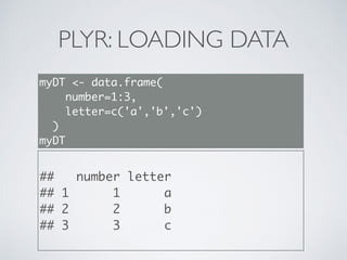
![PLYR: SELECTING COLUMNS
head(D[,c('e_prev_100k','e_prev_100k_lo',
'e_prev_100k_hi')])
## e_prev_100k e_prev_100k_lo e_prev_100k_hi
## 1 306 156 506
## 2 343 178 562
## 3 371 189 614
## 4 392 194 657
## 5 410 198 697
## 6 424 199 733](https://image.slidesharecdn.com/dplyr-slides-150119102051-conversion-gate02/85/Dplyr-and-Plyr-6-320.jpg)

![DPLYR: SELECTING
D %>%
select(e_prev_100k,e_prev_100k_lo,e_prev_100k_hi)
## Source: local data frame [5,120 x 3]
##
## e_prev_100k e_prev_100k_lo e_prev_100k_hi
## 1 306 156 506
## 2 343 178 562
## 3 371 189 614
## 4 392 194 657
## 5 410 198 697
## 6 424 199 733
## 7 438 202 764
## 8 448 203 788
## 9 454 204 800
## 10 446 203 782
## .. ... ... ...](https://image.slidesharecdn.com/dplyr-slides-150119102051-conversion-gate02/85/Dplyr-and-Plyr-20-320.jpg)
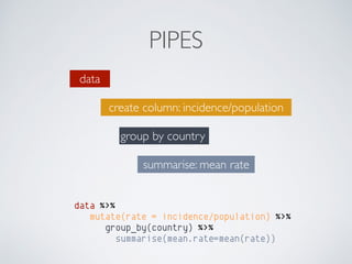
![DPLYR: FILTER & SUMMARISE
D %>%
filter(country == 'Afghanistan') %>%
summarise(
mid=mean(e_prev_100k),
lo=mean(e_prev_100k_lo),
hi=mean(e_prev_100k_hi)
)
## Source: local data frame [1 x 3]
##
## mid lo hi
## 1 376.4 187.2 630.7](https://image.slidesharecdn.com/dplyr-slides-150119102051-conversion-gate02/85/Dplyr-and-Plyr-21-320.jpg)
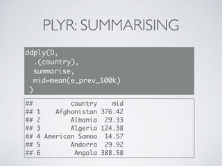
![DPLYR: FILTER & SUMMARISE
D %>%
group_by(country) %>%
summarise(mid=mean(e_prev_100k))
## Source: local data frame [219 x 2]
##
## country mid
## 1 Afghanistan 376.417
## 2 Albania 29.333
## 3 Algeria 124.375
## 4 American Samoa 14.567
## 5 Andorra 29.921
## 6 Angola 388.583
## 7 Anguilla 52.417
## 8 Antigua and Barbuda 8.725
## 9 Argentina 55.500
## 10 Armenia 76.875
## .. ... ...](https://image.slidesharecdn.com/dplyr-slides-150119102051-conversion-gate02/85/Dplyr-and-Plyr-22-320.jpg)
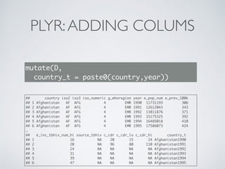
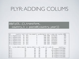
![DPLYR:ADDING COLUMNS
D %>%
mutate(country_t = paste0(country,year)) %>%
select(country_t)
## Source: local data frame [5,120 x 1]
##
## country_t
## 1 Afghanistan1990
## 2 Afghanistan1991
## 3 Afghanistan1992
## 4 Afghanistan1993
## 5 Afghanistan1994
## 6 Afghanistan1995
## 7 Afghanistan1996
## 8 Afghanistan1997
## 9 Afghanistan1998
## 10 Afghanistan1999
## .. ...](https://image.slidesharecdn.com/dplyr-slides-150119102051-conversion-gate02/85/Dplyr-and-Plyr-24-320.jpg)
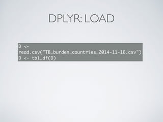
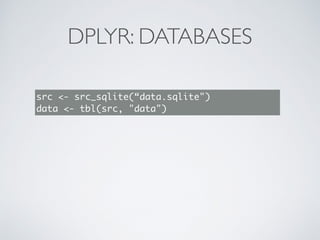
![DPLYR: DATABASES
data <- data.frame(x=1:200000000,
y=runif(4), z=runif(50))
format(object.size(data), units="GB")
## [1] "3.7 Gb"](https://image.slidesharecdn.com/dplyr-slides-150119102051-conversion-gate02/85/Dplyr-and-Plyr-25-320.jpg)
![DPLYR: DATABASES
data %>%
summarise(mean(x), max(y), mean(z))
## Source: sqlite 3.7.17 [data.sqlite]
## From: <derived table> [?? x 3]
##
## mean(x) max(y) mean(z)
## 1 1e+08 0.9008 0.4501
## .. ... ... ...](https://image.slidesharecdn.com/dplyr-slides-150119102051-conversion-gate02/85/Dplyr-and-Plyr-27-320.jpg)
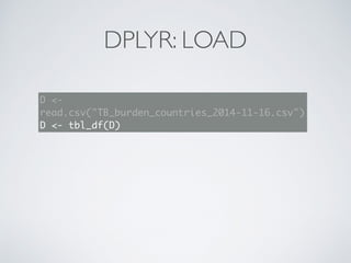
![DPLYR: DATABASES
data %>%
summarise(mean(x), max(y), mean(z))
## Source: sqlite 3.7.17 [data.sqlite]
## From: <derived table> [?? x 3]
##
## mean(x) max(y) mean(z)
## 1 1e+08 0.9008 0.4501
## .. ... ... ...
Use data as if it were local data.frame
Processing done in the database](https://image.slidesharecdn.com/dplyr-slides-150119102051-conversion-gate02/85/Dplyr-and-Plyr-28-320.jpg)


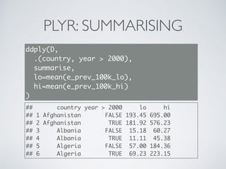
![PLYR: SUMMARISING
library(plyr)
E <- D[with(D, country=='Afghanistan'),]
ddply(E, .(country), summarise,
mid=mean(e_prev_100k),
lo=mean(e_prev_100k_lo),
hi=mean(e_prev_100k_hi) )
## country mid lo hi
## 1 Afghanistan 376.4 187.2 630.7](https://image.slidesharecdn.com/dplyr-slides-150119102051-conversion-gate02/85/Dplyr-and-Plyr-31-320.jpg)
![return data frame
PLYR: SUMMARISING
library(plyr)
E <- D[with(D, country=='Afghanistan'),]
ddply(E, .(country), summarise,
mid=mean(e_prev_100k),
lo=mean(e_prev_100k_lo),
hi=mean(e_prev_100k_hi) )
take data frame](https://image.slidesharecdn.com/dplyr-slides-150119102051-conversion-gate02/85/Dplyr-and-Plyr-32-320.jpg)
![return data frame
PLYR: SUMMARISING
library(plyr)
E <- D[with(D, country=='Afghanistan'),]
ddply(E, .(country), summarise,
mid=mean(e_prev_100k),
lo=mean(e_prev_100k_lo),
hi=mean(e_prev_100k_hi) )
take data frame
grouping columnsinput](https://image.slidesharecdn.com/dplyr-slides-150119102051-conversion-gate02/85/Dplyr-and-Plyr-33-320.jpg)
![return data frame
PLYR: SUMMARISING
library(plyr)
E <- D[with(D, country=='Afghanistan'),]
ddply(E, .(country), summarise,
mid=mean(e_prev_100k),
lo=mean(e_prev_100k_lo),
hi=mean(e_prev_100k_hi) )
take data frame
grouping columnsinput
new columns](https://image.slidesharecdn.com/dplyr-slides-150119102051-conversion-gate02/85/Dplyr-and-Plyr-34-320.jpg)
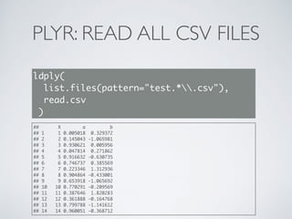
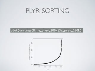
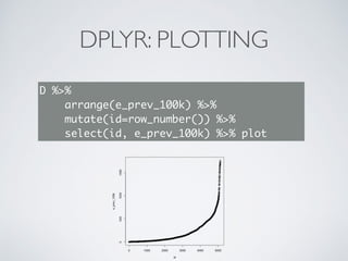
![PLYR: PLOT EACH GROUP
d_ply(
long,
.(Sensor),
function(df){
pdf(paste0(df$Sensor[1],".pdf"));
plot(df$value);
dev.off()
})](https://image.slidesharecdn.com/dplyr-slides-150119102051-conversion-gate02/85/Dplyr-and-Plyr-36-320.jpg)


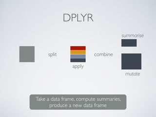
The document discusses the use of the R packages plyr and dplyr for data manipulation. It covers various data operations such as loading, filtering, summarizing, and adding columns to data frames, particularly focusing on tuberculosis burden data. Key examples illustrate the methods for calculating mean values and creating new variables through data transformations.


![Introduction to Pandas and Time Series Analysis [PyCon DE]](https://cdn.slidesharecdn.com/ss_thumbnails/introductiontopandasandtimeseriesanalysispyconde-170617163724-thumbnail.jpg?width=640&height=640&fit=bounds)