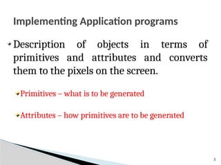
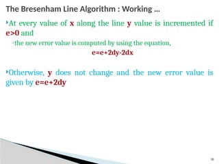
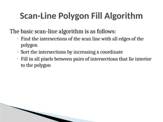
Output primitives are the fundamental building blocks in computer graphics for creating images, serving as basic geometric shapes like points, lines, and polygons. They are the simplest graphical elements that a system can directly render to a display device. These primitives have attributes that control their appearance, such as color, width, and type (for lines), and are processed by the Graphics Processing Unit (GPU) to form more complex visuals
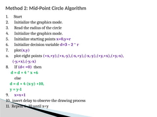
![23
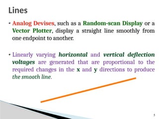
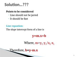
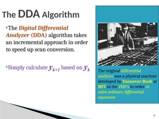
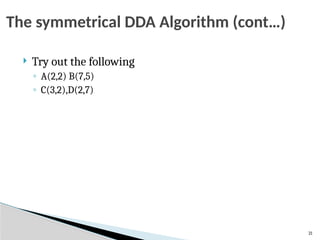
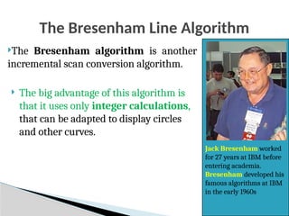
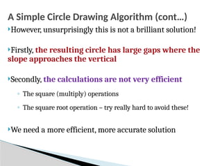
The simple DDA Algorithm
1. Input the 2 endpoints (x1,y1) and (x2,y2)
2. Calculate the constants dx and dy
dx= x2-x1 and dy= y2-y1
3. [Obtain the length(or the number of steps)]
if (abs(dx)> abs(dy)) then
length=abs(dx)
else
length=abs(dy)
4. [Determine the increment values of x and y]
xinc =dx/length and yinc =dy/length](https://image.slidesharecdn.com/0202outputprimitives-251009063030-d20d70ff/85/Output-Primitives-in-Computer-Graphics-pptx-23-320.jpg)
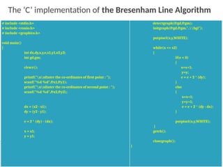
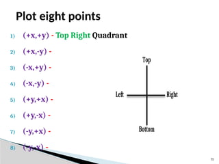
![24
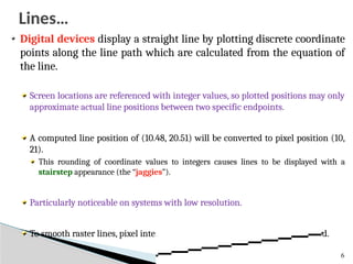
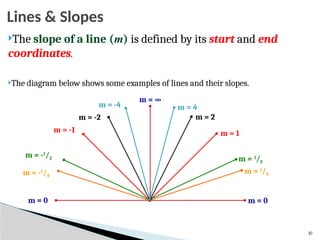
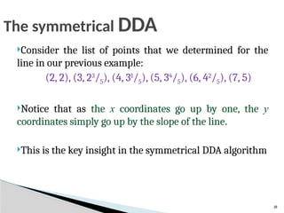
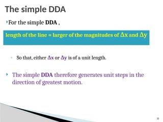
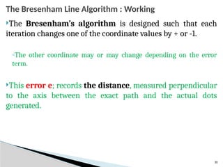
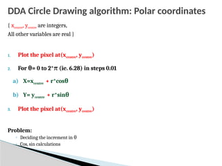
The simple DDA Algorithm
5. Plot the starting point
6. For i=1 to length[i=i+1]
7. [Plot the next point by generating it]
x=x+xinc
y=y+yinc
[End FOR]
8. Stop](https://image.slidesharecdn.com/0202outputprimitives-251009063030-d20d70ff/85/Output-Primitives-in-Computer-Graphics-pptx-24-320.jpg)

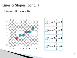
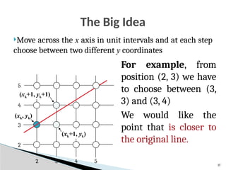
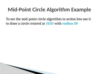
![27
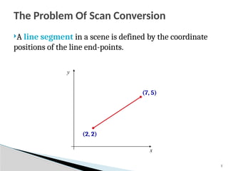
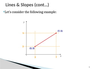
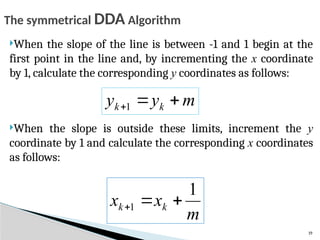
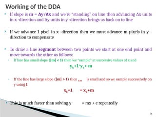
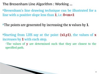
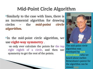
The DDA Algorithm Summary
Walk through the line, starting at (x0,y0)
◦ Constrain x, y increments to values in [0,1] range
◦ Case a: x is incrementing faster (m < 1)
Step in x=1 increments, compute and round y
◦ Case b: y is incrementing faster (m > 1)
Step in y=1 increments, compute and round x](https://image.slidesharecdn.com/0202outputprimitives-251009063030-d20d70ff/85/Output-Primitives-in-Computer-Graphics-pptx-27-320.jpg)
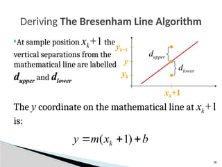
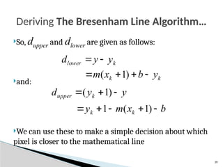
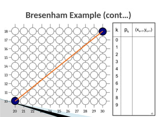
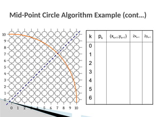
![34
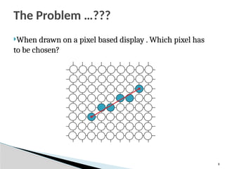
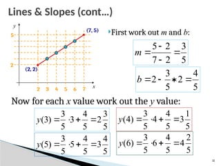
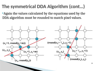
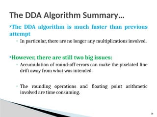
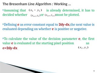
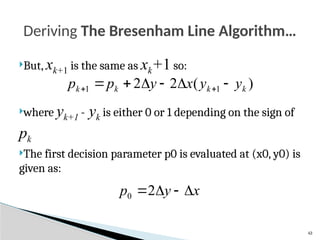
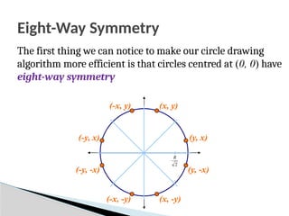
1. [Input] endpoints (x1,y1) and (x2,y2)
2. [Calculate] dx=x2-x1 and dy=y2-y1
3. [Obtain starting decision parameter] e=2dy-dx
4. If (x2>x1)then
x=x1,
y=y1,
xend=x2
Else
x=x2,
y=y2,
xend=x1
[End If]
The Bresenham Line Algorithm for |m|<1](https://image.slidesharecdn.com/0202outputprimitives-251009063030-d20d70ff/85/Output-Primitives-in-Computer-Graphics-pptx-34-320.jpg)
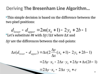
![35
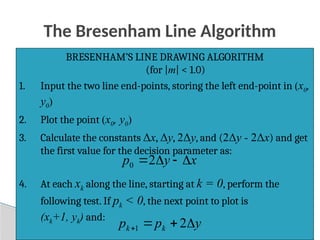
5. While (x<xend)
6. If (e>0)then
y=y+1
e=e+2(dy-dx)
Else
e=e+2dy [End if]
7. x=x+1
[End while]
8. Stop
The Bresenham Line Algorithm for |m|<1](https://image.slidesharecdn.com/0202outputprimitives-251009063030-d20d70ff/85/Output-Primitives-in-Computer-Graphics-pptx-35-320.jpg)
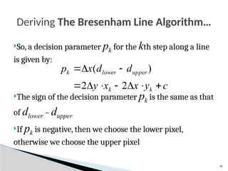
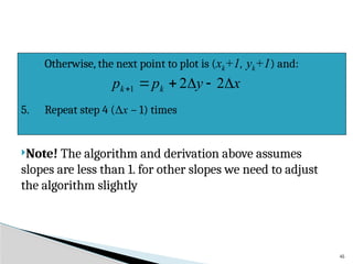

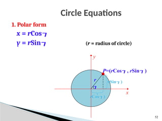
![Drawing a circle
53
Disadvantages
To find a complete circle varies from 0° to 360°
The calculation of trigonometric functions is very slow.
= 0°
while ( < 360°)
x = rCos
y = rSin
setPixel(x,y)
= + 1°
[End while]](https://image.slidesharecdn.com/0202outputprimitives-251009063030-d20d70ff/85/Output-Primitives-in-Computer-Graphics-pptx-53-320.jpg)
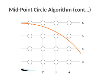
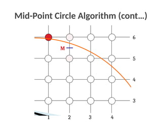
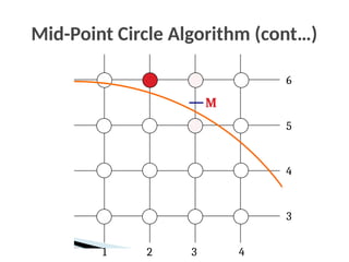
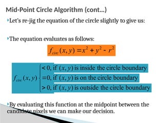
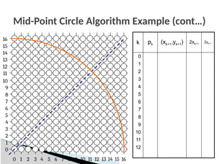
![Mid-Point Circle Algorithm (cont…)
To ensure things are as efficient as possible we can do all of
our calculations incrementally
First consider:
Or:
where yk+1 is either yk or yk-1 depending on the sign of pk
2
2
1
2
1
1
1
2
1
]
1
)
1
[(
2
1
,
1
r
y
x
y
x
f
p
k
k
k
k
circ
k
1
)
(
)
(
)
1
(
2 1
2
2
1
1
k
k
k
k
k
k
k y
y
y
y
x
p
p](https://image.slidesharecdn.com/0202outputprimitives-251009063030-d20d70ff/85/Output-Primitives-in-Computer-Graphics-pptx-67-320.jpg)
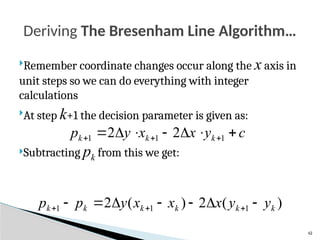
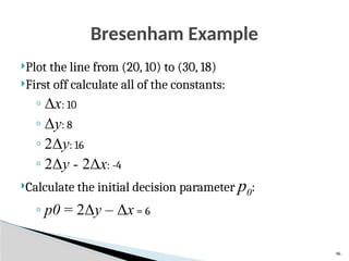
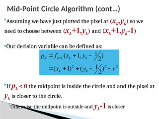
![The Mid-Point Circle Algorithm
1. [Input] radius r and circle centre (xc, yc), then set the coordinates for
the first point on the circumference of a circle centred on the
origin as:
2. [Calculate] the initial value of the decision parameter as:
3. Starting with k = 0 at each position xk, perform the following test. If
pk < 0, the next point along the circle centred on (0, 0) is (xk+1, yk)
and:
)
,
0
(
)
,
( 0
0 r
y
x
r
p
4
5
0
1
2 1
1
k
k
k x
p
p](https://image.slidesharecdn.com/0202outputprimitives-251009063030-d20d70ff/85/Output-Primitives-in-Computer-Graphics-pptx-69-320.jpg)


![Chapter 3 - Part 1 [Autosaved].pptx](https://cdn.slidesharecdn.com/ss_thumbnails/chapter3-part1autosaved-230109040832-9344385c-thumbnail.jpg?width=640&height=640&fit=bounds)


![5G Explained! A High Level Overview [Introduction]](https://cdn.slidesharecdn.com/ss_thumbnails/5gexplainedahighleveloverview-260119165306-cc137a3e-thumbnail.jpg?width=640&height=640&fit=bounds)


