The document describes algorithms for scan converting lines and circles in raster graphics. For line drawing, it discusses direct solutions, the digital difference analyzer (DDA) algorithm, and the midpoint line algorithm. The midpoint line algorithm uses incremental calculations and the sign of a decision variable to determine whether to select the east or northeast pixel at each step. For circle drawing, it describes using the implicit equation and symmetry to scan convert circles centered at the origin. It then presents the midpoint circle algorithm, which similarly uses a decision variable and incremental updates to select between the east and southeast pixels at each step.

1. SCAN CONVERTING
LINES,
CIRCLES and ELLIPSES

2. LINE DRAWING
Description: Given the specification for a
straight line, find the collection of
addressable pixels which most closely
approximates this line.
Goals (not all of them are achievable with
the discrete space of a raster device):
• Straight lines should appear straight.
• Lines should start and end accurately,
matching endpoints with connecting lines.
• Lines should have constant brightness.
• Lines should be drawn as rapidly as possible.

3. Problems:
 How do we determine which pixels to
illuminate to satisfy the above goals?
 Vertical, horizontal, and lines with slope
= +/- 1, are easy to draw.
 Others create problems: stair-casing/
jaggies/aliasing.
 Quality of the line drawn depends on the
location of the pixels and their brightness

4. It is difficult to determine whether
a pixel belongs to an object

5. Direct Solution:
Solve y=mx+b, where (0,b) is the y-intercept
and m is the slope.
Go from x0 to x1:
calculate round(y) from the equation.
Take an example, b = 1 (starting point (0,1))
and m = 3/5.
Then x
x
x
x
x
=
=
=
=
=
1,
2,
3,
4,
5,
y
y
y
y
y
=
=
=
=
=
2
2
3
3
4
=
=
=
=
=
round(8/5)
round(11/5)
round(14/5)
round(17/5)
round(20/5)
For results, see next slide.

6. (5,4)
4
3
2
(0,1) 1
2
3
4
5
Ideal Case of a line drawn in a graph paper

7. Choice of pixels in the raster, as integer values
x = 1, y = 2 = round(8/5)
x = 2, y = 2 = round(11/5)
x = 3, y = 3 = round(14/5)
x = 4, y = 3 = round(17/5)
x = 5, y = 4 = round(20/5)
Using next highest
4
3
2
(0,1)
(5,4)
Using Round
4
3
2
(0,1)
(5,4)

8. Why is this undesired?
• `*´ and `/´ are expensive
• Round() function needed
• Can get gaps in the line (if slope > 1)
Take another example:
y = 10.x + 2
x=1, y=12;
x=2, y=22.

9. DDA - Digital Difference Analyzer
Incremental Algorithm.
Based on y = (y1- y0) / (x1-x0) x + b
Assume x1 > x0 and |dx| > |dy|
(can be easily modified for the other
cases.)
The Algorithm: dx = x1- x0 ;
dy = y1- y0 ;
m = dy/dx ;
y = y0 ;
for (x=x0 to x1)
draw_point (x, round(y)) ;
y=y+m;
end for

10. Problems:
Still uses floating point and round()
inside the loop.
How can we get rid of these?

11. Octants covering the 2-D space
3
2
4
1
5
8
6
7

12. MIDPOINT LINE ALGORITHM
Incremental Algorithm (Assume first octant)
Given the choice of the current pixel,
which one do we choose next : E or NE?
Equations:
1. y = (dy/dx) * x + B
Rewrite as:
2. F(x,y) = a*x + b*y + c = 0
Gives: F(x,y) = dy*x - dx*y + B*dx = 0
=> a = dy, b = -dx, c = B*dx

13. Criteria:
Evaluate the mid-point, M,
w.r.t. the equation of the line.
Choice: E or NE?
NE
E
M
F(x,y) = dy*x - dx*y + B*dx =0
F(x,y) > 0; if point below the line
F(x,y) < 0; if point above the line

14. NE (Xp+1, Yp+1)
Q
M
(Xp+1, Yp+1/2)
E
(Xp, Yp)
(Xp+1, Yp)
Q is above M,
hence select NE pixel as your next choice

15. NE (Xp+1, Yp+1)
M (Xp+1, Yp+1/2)
Q
E
(Xp, Yp)
(Xp+1, Yp)
Q is below M, hence
select E pixel as
your next choice
ALGO – for next choice:
If F(M) > 0 /*Q is above M */
then Select NE
/*M is below the line*/
else Select E ;
/* also with F(M) = 0 */

16. Evaluate mid-point M using a decision
variable d = F(X,Y);
d = F(Xp+1,Yp+1/2) = a(Xp+1)+b(Yp+1/2)+c;
at M,
Set dold = d;
Based on the sign of d, you choose E or NE.
Case I. Chosen E:
dnew = F(Xp+2,Yp+1/2)
= a(Xp+2) + b(Yp+1/2) + c
(d)E = dnew - dold = a
/* = dy */

17. NE (Xp+1, Yp+1)
Q
Case II.
Chosen NE:
M
(Xp+1, Yp+1/2)
E
(Xp, Yp)
(Xp+1, Yp)
dnew = F(Xp+2,Yp+3/2)
= a(Xp+2) + b(Yp+3/2) + c
(d)NE = dnew - dold = a + b /*= dy – dx */
Update using dnew = dold + d

18. Midpoint criteria
d = F(M) = F(Xp+1, Yp+1/2);
if d > 0 choose NE
else /* if d <= 0 */ choose E ;
Case EAST :
increment M by 1 in x
dnew= F(Mnew) = F(Xp + 2, Y + 1/2)
(d)E = dnew - dold = a = dy
(d)E = dy
Case NORTH-EAST:
increment M by 1 in both x and y
dnew= F(Mnew) = F(Xp + 2, Yp + 3/2)
(d)NE = dnew - dold = a + b = dy - dx
(d)NE = dy - dx

19. What is dstart?
dstart = F(x0 + 1, y0 + 1/2)
= ax0 + a + by0 + b/2 + c
= F(x0, y0)+ a + b/2
= dy - dx/2
Let's get rid of the fraction and see what
we end up with for all the variables:
dstart
= 2dy – dx ;
(d)E
= 2dy ;
(d)NE = 2(dy - dx) ;

20. The Midpoint Line Algorithm
x
= x0;
y
dy = y1 - y0 ;
d
= y0;
dx = x1 - x0;
= 2dy – dx;
(d)E = 2dy;
(d)NE = 2(dy - dx);
Plot_Point(x,y)

21. The Midpoint Line Algorithm (Contd.)
while (x < x1)
if (d <= 0) /* Choose E */
d = d + (d)E ;
else
/* Choose NE */
d = d + (d)NE ;
y=y+1
endif
x=x+1;
Plot_Point(x, y) ;
end while

22. Example:
INIT: dy = 3; dx = 4; dstart=2;
Starting point:
(5, 8)
Ending point:
(9, 11)
(d)E = 6;
Successive
steps:
(d)NE = -2;
11
13
12
10
• d=2, (6, 9)
9
• d=0, (7, 9)
8
• d=6, (8, 10)
7
• d=4, (9, 11)
6
4
5
6
7
8
9 10 11

23. We have considered lines in the first
Quadrant only.
What about
the rest?
3
2
4
1
5
8
6
7

24. How do you generalize this to the other
octants?
Octant
Change
1
none
2
Switch roles of x & y
3
Switch roles of x & y; Use (4)
4
Draw from P1 to P0; Use (8)
5
Draw from P1 to P0
6
Draw from P1 to P0; Use (2)
7
Switch roles of x & y; Use (8)
8
Use y = y - 1.

25. 3
2
4
Octant
1
Change
None
1
5
8
6
2
Switch roles of x & y
3
Switch roles of x & y; Use (4)
4
Draw from P1 to P0; Use (8)
5
Draw from P1 to P0
6
Draw from P1 to P0; Use (2)
7
Switch roles of x & y; Use (8)
8
Use y = y - 1.
7

26. Draw from P1 to P0:
swap(P0, P1).
Use y = y - 1;
dy = -dy;
Switch Roles of X & Y:
Swap (x1, y1);
Swap (x0, y0 );
Swap (dx, dy);
plot_point(y, x);

27. 12
11
10
9
8
7
6
Issues: Staircasing,
Fat lines, end-effects
and end-point ordering.
4 5 6 7 8 9 10

28. ANTI-ALIASING
5
4
3
2
1
0
0
1
2
3
4
5
6
7
8
9 10 11

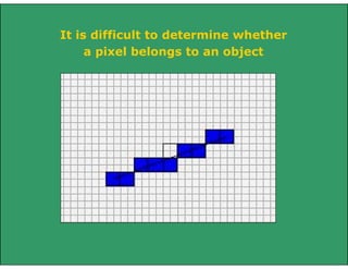
29. X=Xmin
NE
[Xmin, round(m.Xmin + b)]
P
[Xmin, m.Xmin + b]
M
E
Q
Y=Ymin
Intersection of a line with a vertical
edge of the clip rectangle

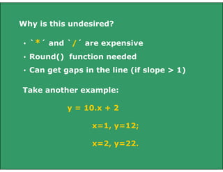
30. X=Xmin
NE
[Xmin, round(m.Xmin + b)]
P
E
[Xmin, m.Xmin + b]
M
Q
Y=Ymin
No problem in this case to round off the
starting point, as that would have been a point
selected by mid-point criteria too.
Select P by rounding the intersection point
coordinates at Q.

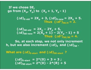
31. X=Xmin
NE
[Xmin, round(m.Xmin + b)]
P
E
[Xmin, m.Xmin + b]
Q
M
Y=Y
min
What about dstart?
If you initialize the algorithm from P, and
then scan convert, you are basically changing “dy”
and hence the original slope of the line.
Hence, start by initializing from d(M), the
mid-point in the next column, (Xmin+ 1), after
clipping).

32. X=Xmin
Y=Ymin
B
A
Y=Ymin-1
Intersection of a shallow line with a
horizontal edge of the clip rectangle

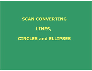
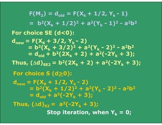
33. Intersection of line with edge and then
rounding off produces A, not B.
To get B, as a part of the clipped line:
Obtain intersection of line with (Ymin - 1/2)
and then round off, as
B = [round(X|Ymin-1/2), Ymin]

34. CIRCLE DRAWING

35. CIRCLE DRAWING

36. Assume second octant
Xp, Yp
E
M
ME
SE
MSE
Now the choice is between pixels E and SE.

37. CIRCLE DRAWING
Only considers circles centered at the origin
with integer radii.
Can apply translations to get non-origin
centered circles.
Explicit equation: y = +/- sqrt(R2 - x2)
Implicit equation: F(x,y)= x2 + y2 - R2 =0
Note: Implicit equations used extensively
for advanced modeling
(e.g., liquid metal creature from
"Terminator 2")

38. Use of Symmetry: Only need to calculate one
octant. One can get points in the other 7
octants as follows:
Draw_circle(x, y)
begin
Plotpoint (x, y); Plotpoint (y, x);
Plotpoint (x, -y); Plotpoint (-y, x);
Plotpoint (-x, -y) ; Plotpoint (-y, -x);
Plotpoint (-x, y); Plotpoint (-y, x);
end

39. (-X, Y)
(X, Y)
(-Y, X)
(Y, X)
(-Y, X)
(-Y, -X)
(-X, -Y)
(X, -Y)

40. MIDPOINT CIRCLE ALGORITHM
Will calculate points for the second octant.
Use draw_circle procedure to calculate the rest.
Now the choice is between pixels E and SE.
F(x, y) = x2 + y2 - R2 =0
F(x, y) > 0 if point is outside the circle
F(x, y) < 0 if point inside the circle.
Again, use dold = F(M) ;
F(M) = F(Xp + 1, Yp - 1/2)
= (Xp + 1)2 + (Yp - 1/2)2 - R2

41. d >= 0 choose SE ; next midpoint: Mnew;
Increment + 1 in X, -1 in y; which gives dnew.
d < 0 choose E ; next midpoint: Mnew;
Increment + 1 in X; which gives = dnew.
(d)SE = dnew – dold
= F(Xp + 2, Yp - 3/2) - F(Xp + 1, Yp - 1/2)
= 2Xp – 2Yp + 5 ;
(d)E = dnew – dold
=F(Xp + 2, Yp - 1/2) - F(Xp + 1, Yp - 1/2)
= 2Xp + 3;
dstart = F(X0 + 1, Y0 - 1/2) = F(1, R - 1/2)
= 1 + (R - 1/2)2 - R2 = 1 + R2 - R + 1/4 - R2
= 5/4 - R

42. Xp, Yp
E
M
ME
SE
MSE
To get rid of the fraction,
Let h = d - ¼
=> hstart = 1 - R
Comparison is: h < -1/4.
Since h is initialized to and incremented
by integers, so we can just do with: h < 0.

43. The Midpoint Circle algorithm:
(Version 1)
x = 0;
y = R;
h = 1 – R;
DrawCircle(x, y);
while (y > x)
if h < 0 /* select E */
h = h + 2x + 3;

44. else
endif
/* select SE */
h = h + 2(x - y) + 5;
y = y - 1;
x = x + 1;
DrawCircle(x, y);
end_while

45. 0
Example:
R = 10;
1
2
3
4
5
6
7
8
10
Initial Values:
h = 1 – R = -9;
X = 0; Y = 10;
2X = 0;
2Y = 20.
9
8
7
6
K
1
2
3
4
5
6
7
h
-6
-1
6
-3
8
5
6
2X
0
2
4
6
8
10
12
2Y
20
20
20
20
18
18
16
(2, 10)
(3, 10)
(4, 9)
(5, 9)
(6, 8)
(7, 7)
X, Y (1, 10)

46. Problems with this?
Requires at least 1 multiplication and
3 additions per pixel.
Why? Because (d)E and (d)SE
are linear functions and not constants.
Solution?
All we have to do is calculate the
differences for: (d)E and dSE (check if these
will be constants). Say, (d2)E and (d2)SE.
If we chose E, then we calculate (d2)E/E
and (d2)E/SE, based on this. Same if we choose
SE, then calculate (d2)SE/E and (d2)SE/SE.

47. If we chose E, go from (Xp, Yp) to (Xp + 1, Yp)
(d)E-old = 2Xp + 3, (d)E-new = 2Xp + 5.
Thus (d2)E/E = 2.
(d)SE-old = 2Xp – 2Yp + 5,
(d)SE-new = 2(Xp + 1) – 2Yp + 5
Thus (d2)E/SE = 2.

48. If we chose SE,
go from (Xp, Yp) to (Xp + 1, Yp - 1)
(d)E-old = 2Xp + 3, (d)E-new = 2Xp + 5.
Thus (d2)SE/E = 2.
(d)SE-old = 2Xp – 2Yp + 5,
(d)SE-new = 2(Xp + 1) – 2(Yp - 1) + 5
Thus (d2)SE/SE = 4.
So, at each step, we not only increment
h, but we also increment (d)E and (d)SE .
What are (d)E-start and (d)SE-start ?
(d)E-start = 2*(0) + 3 = 3 ;
(d)SE-start = 2*(0) - 2*(R) + 5

49. The MidPoint Circle Algorithm
(Version 2):
x = 0;
h=1–R;
deltaE = 3 ;
y = radius;
deltaSE = -2*R + 5 ;
DrawCircle(x, y);
while (y > x)
if h < 0
/* select E */
h = h + deltaE ;
deltaE = deltaE + 2;
deltaSE= deltaSE + 2

50. else
/* select SE */
h = h + deltaSE ;
deltaE = deltaE + 2 ;
deltaSE = deltaSE + 4
y=y–1;
endif
x=x+1;
DrawCircle(x, y) ;
end_while

51. 0
Example:
R = 10;
10
Initial Values:
9
X = 0; Y = 10;
h = 1 – R = -9; 8
E = 3;
SE = -15;
1
2
3
4
5
6
7
8
7
6
K
1
2
3
4
5
6
7
h
-6
-1
6
-3
8
5
6
E
5
7
9
11
13
15
17
SE
-13
-11
-9
-5
-3
1
5
(2, 10)
(3, 10)
(4, 9)
(5, 9)
(6, 8)
(7, 7)
X, Y (1, 10)

52. Comparison of the solutions with two different methods
K
1
2
3
4
5
6
7
h
-6
-1
6
-3
8
5
6
E
5
7
9
11
13
15
17
SE
-13
-11
-9
-5
-3
1
5
(4, 9)
(5, 9)
(6, 8)
(7, 7)
X, Y (1, 10)
(2, 10) (3, 10)
K
1
2
3
4
5
6
7
h
-6
-1
6
-3
8
5
6
2X
0
2
4
6
8
10
12
2Y
20
20
20
20
18
18
16
(2, 10)
(3, 10)
(4, 9)
(5, 9)
(6, 8)
(7, 7)
X, Y (1, 10)

53. ELLIPSE DRAWING

54. SCAN CONVERTING ELLIPSES
b
Y
-a
a
Equation of Ellipse
centered at origin:
-b
F(X,Y)  b X  a Y  a b  0
2
2
2
2
2
2
Length of the major axis: 2a;
and minor axis: 2b.
X

55. Y
R1
slope = -1
R2
X
Draw pixels in two regions R1 and R2,
to fill up the first Quadrant.
Points in other quadrants are obtained
using symmetry.

56. We need to obtain the point on the
contour where the slope of the curve is -1.
This helps to demarcate regions R1 and R2.
The choice of pixels in R1 is between E and SE,
whereas in R2, it is S and SE.
F(X,Y)  b X  a Y  a b  0
2
2
f
f
In R1 :

 Y X
and
f
f
in R2 :

X Y
2
2
Y
R1
2
2
f ˆ f ˆ
grad f X, Y 
i
j
X
Y
 (2b2 X) ˆ  (2a2 Y) ˆ
i
j
slope = -1
R2
X

57. At the region boundary point on the ellipse:
f
f

X
Y
Based on this condition,
we obtain the criteria when the next mid-point
moves from R1 to R2 :
b (X p  1)  a (Y p  1/2)
2
2
When the above condition occurs,
we switch from R1 to R2.
Analysis in region R1:
Let the current pixel be (Xp, Yp);
dold = F(M1);

58. F(M1) = dold = F(Xp + 1, Yp - 1/2)
= b2(Xp + 1)2 + a2(Yp - 1/2)2 - a2b2
For choice E (d<0):
dnew = F(Xp + 2, Yp - 1/2)
= b2(Xp + 2)2 + a2(Yp - 1/2)2 - a2b2
= dold + b2(2Xp + 3);
For choice SE (d>0):
Thus, (d)E1 = b2(2Xp + 3);
dnew = F(Xp + 2, Yp - 3/2)
= b2(Xp + 2)2 + a2(Yp - 3/2)2 - a2b2
= dold + b2(2Xp + 3) + a2(-2Yp + 2) ;
Thus, (d)SE1 = b2(2Xp + 3) + a2(-2Yp + 2) ;

59. Initial Condition:
In region R1, first point is (0, b).
(dinit)R1 = F(1, b - 1/2) = b2 + a2(1/4 - b) ;
Problem with a fractional (floating point) value
for (dinit)R1 ?
Switch to Region R2, when:
b (X p  1)  a (Y p  1/2)
2
2
Let the last point in R1 be (Xk, Yk).
F(M2) = F(Xk + 1/2, Yk - 1)
= b2(Xk + 1/2)2 + a2(Yk - 1)2 - a2b2
= (dinit)R2

60. F(M2) = dold = F(Xk + 1/2, Yk - 1)
= b2(Xk + 1/2)2 + a2(Yk - 1)2 - a2b2
For choice SE (d<0):
dnew = F(XK + 3/2, Yk - 2)
= b2(Xk + 3/2)2 + a2(Yk - 2)2 - a2b2
= dold + b2(2Xk + 2) + a2(-2Yk + 3);
Thus, (d)SE2 = b2(2Xk + 2) + a2(-2Yk + 3);
For choice S (d>0):
dnew = F(XK + 1/2, Yk - 2)
= b2(Xk + 1/2)2 + a2(Yk - 2)2 - a2b2
= dold + a2(-2Yk + 3);
Thus, (d)S2 = a2(-2Yk + 3);
Stop iteration, when Yk = 0;

61. void MidPointEllipse (int a, int b, int value);
{
double d2; int X = 0; int Y = 0;
sa = sqr(a); sb = sqr(b);
double d1 = sb – sa*b + 0.25*sa;
EllipsePoints(X, Y, value);
/* 4-way symmetrical pixel plotting */
while ( sa*(Y - 0.5) > sb*(X + 1))
/*Region R1 */
{
if (d1 < 0)
/*Select E */
d1 += sb*((X<<1) + 3);
else
/*Select SE */
{ d1 += sb*((X<<1) + 3) + sa*
(-(Y<<1) + 2); Y-- ; }
X++ ; EllipsePoints(X, Y, value);
}

62. double d2 = sb*sqr(X + 0.5) +
sa*sqr(Y - 1) - sa*sb;
while ( Y > 0)
{
if (d2 < 0)
/*Select SE */
{ d2 += sb*((X<<1) + 2) +
sa*(-(Y<<1) + 3);
X++; }
else
}
}
/*Region R2 */
/*Select S */
d2 += sa*(-(Y<<1) + 3);
Y-- ; EllipsePoints(X, Y, value);

63. In some cases the quality of
the picture is not satisfactory