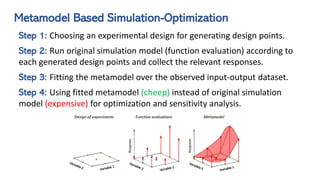
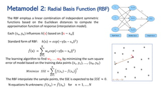
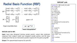
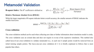
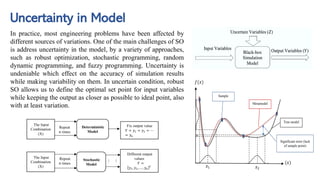
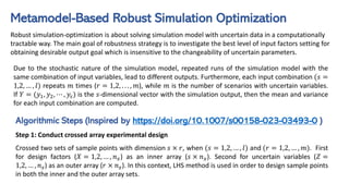
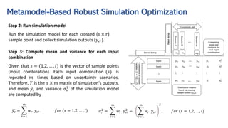
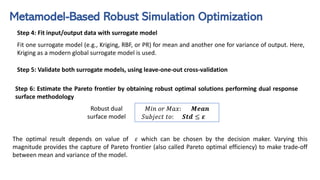
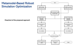
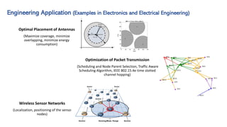
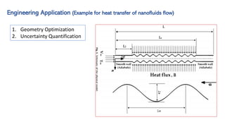
The document provides biographical and research information about Amir Parnianifard. It summarizes his educational background, current affiliations with Glasgow College and the University of Electronic Science and Technology of China, and contact information. It then lists his main research interests as engineering design optimization, surrogate modeling, uncertainty quantification, and other topics in computational intelligence and optimal control. The document provides an overview of differential evolution algorithms and includes MATLAB code examples for implementing differential evolution optimization and other related modeling techniques.


![Eng. Optimization using Evolutionary Algorithms
➢ In computational intelligence, an Evolutionary
Algorithm (EA) is a subset of evolutionary
computation, a generic population-based
metaheuristic optimization algorithm. An EA uses
mechanisms inspired by biological evolution, such as
reproduction, mutation, recombination, and
selection.
➢ Genetic Algorithm (GA) is the most popular type of
EA. A search heuristic known as a genetic algorithm
was motivated by Charles Darwin's theory of natural
selection[57], [58].
➢ Differential Evolution (DE) is based on vector
differences and is therefore primarily suited for
numerical optimization problems.](https://image.slidesharecdn.com/cibasdoptimization-amirparnianifard-230608071414-6463fe26/85/Computational-Intelligence-Assisted-Engineering-Design-Optimization-using-MATLAB-4-320.jpg)
![DE Optimizer (MATLAB Code)
Input: Fitness function of problem, Lower and Upper limits of design variables, Number of Initial Papulation,
and Maximum Number of Iteration by Algorithm
Output: The Optimum results for design variables and the relevant fitness function (in the optimum point).
function [Opt_var,Opt_cost] = DEO(objFcn,LoB,UpB,NoPapulation,MaxIteration)
% This is the code for Differential evolution (DE)
%% Parameter Adjustement
nVar = length(LoB);
CR = 0.5; % Crossover Rate
FF = 1-exp(-norm(0.05*(UpB-LoB)))* rand();
%Initial Papulation
individuals = (UpB-LoB).*rand(NoPapulation ,nVar) + LoB;
% figure('Position', [400, 400, 800, 300]); hold on
%% Optimization
for iter = 1 : MaxIteration
for i = 1:NoPapulation
ind0 = individuals;
ind0(i,:) = [];
X = individuals(i,:);
Cost_X = objFcn(X);
cost(i,1) = Cost_X;
var_X(i,:) = X;
idx = randperm(NoPapulation-1,3);
X1 = ind0(idx(1),:);
X2 = ind0(idx(2),:);
X3 = ind0(idx(3),:);
d_rand = randperm(nVar,1);
for d = 1:nVar
if d == d_rand || rand <= CR
u(d) = X1(d) + FF *rand()* (X2(d) - X3(d));
if u(d) < LoB(d) || u(d) > UpB(d)
u(d) = (UpB(d) - LoB(d))/2 + LoB(d);
end
else
u(d) = X(d);
end
end
if objFcn(u) < Cost_X
individuals(i,:) = u;
end
end
[best_cost(iter),nr] = min(cost);
best_var(iter,:) = var_X(nr,:);
end
[Opt_cost,nr] = min(best_cost);
Opt_var = best_var(nr,:);
end](https://image.slidesharecdn.com/cibasdoptimization-amirparnianifard-230608071414-6463fe26/85/Computational-Intelligence-Assisted-Engineering-Design-Optimization-using-MATLAB-6-320.jpg)
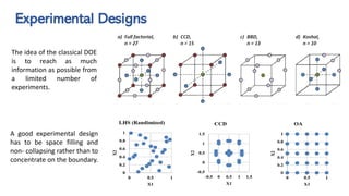
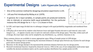
![Latin Hypercube Sampling (LHS)
function [LHS_Samp] = LHS_Design(NSamp,MinRangeSamp,MaxRangeSamp,Type)
[~,NVar]=size(MinRangeSamp);
switch Type
case 'maximin'
Train_lhs = lhsdesign(NSamp,NVar,'criterion','maximin');
case 'none'
Train_lhs = lhsdesign(NSamp,NVar,'criterion','none');
case 'correlation'
Train_lhs = lhsdesign(NSamp,NVar,'criterion','correlation');
end
LHS_Samp=[];
for sa = 1:NSamp
for va = 1:NVar
L = MinRangeSamp(1,va);
U = MaxRangeSamp(1,va);
X = Train_lhs(sa,va)*(U-L)+L;
XR(1,va) = X;
end
LHS_Samp = [LHS_Samp;XR];
end
end
Note: the MATLAB® function “lhsdesign”
is located in Deep Learning Toolbox.
Make sure install Deep Learning
Toolbox.
Input: Number of sample points, Lower
and Upper bound for design variables,
and type of LHS.
Output: Designed sample points in
upper and lower range.
MATLAB® code](https://image.slidesharecdn.com/cibasdoptimization-amirparnianifard-230608071414-6463fe26/85/Computational-Intelligence-Assisted-Engineering-Design-Optimization-using-MATLAB-11-320.jpg)


![[DL輪読会]SurfelGAN: Synthesizing Realistic Sensor Data for Autonomous Driving](https://cdn.slidesharecdn.com/ss_thumbnails/surfelgan-200710035231-thumbnail.jpg?width=640&height=640&fit=bounds)