This document provides an introduction to digital control systems. It discusses how control systems consisting of interconnected components can be designed to achieve a desired purpose. Modern control engineering uses digital control strategies to improve various processes. The design gap exists between physical systems and their models. The iterative nature of design allows engineers to effectively handle this gap. Digital control offers advantages over analog control like accuracy, flexibility and lower costs. However, digital control can introduce delays. Examples of digitally controlled systems include automotive engine control and aircraft autopilots. Controller design involves modeling systems, transforming between differential and difference equations, and mapping between the s-plane and z-plane.
Introduction to digital control systems, presented by Prof. Dr. Khalaf S Gaeid from Tikrit University.
Control systems comprise interconnected components for achieving objectives in industry and modeling, addressing design gaps.
Digital control refers to implementing control laws via digital devices, offering advantages like accuracy, flexibility, and cost-effectiveness.
Despite its benefits, digital control may introduce delays in the feedback loop compared to analog control.
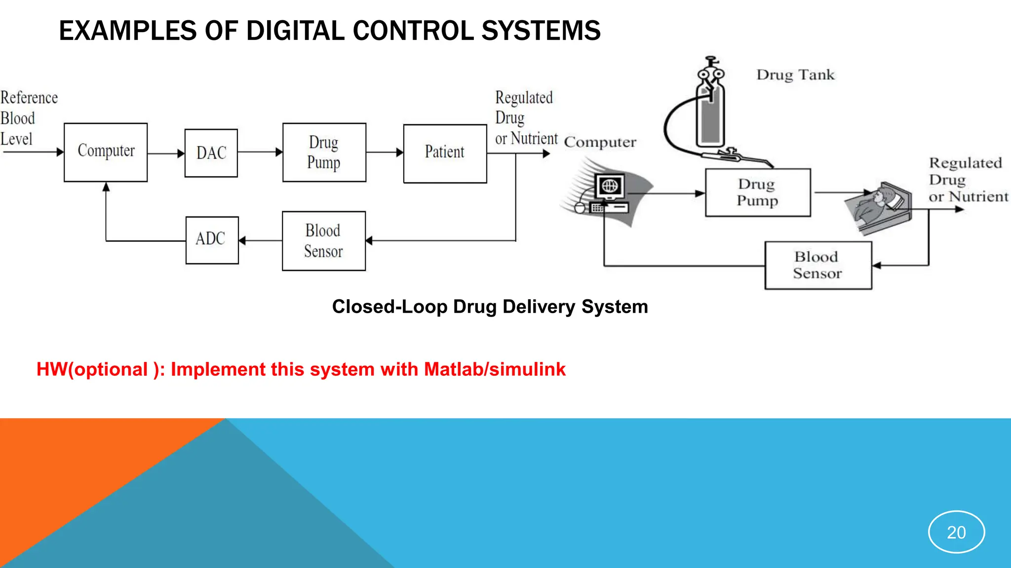
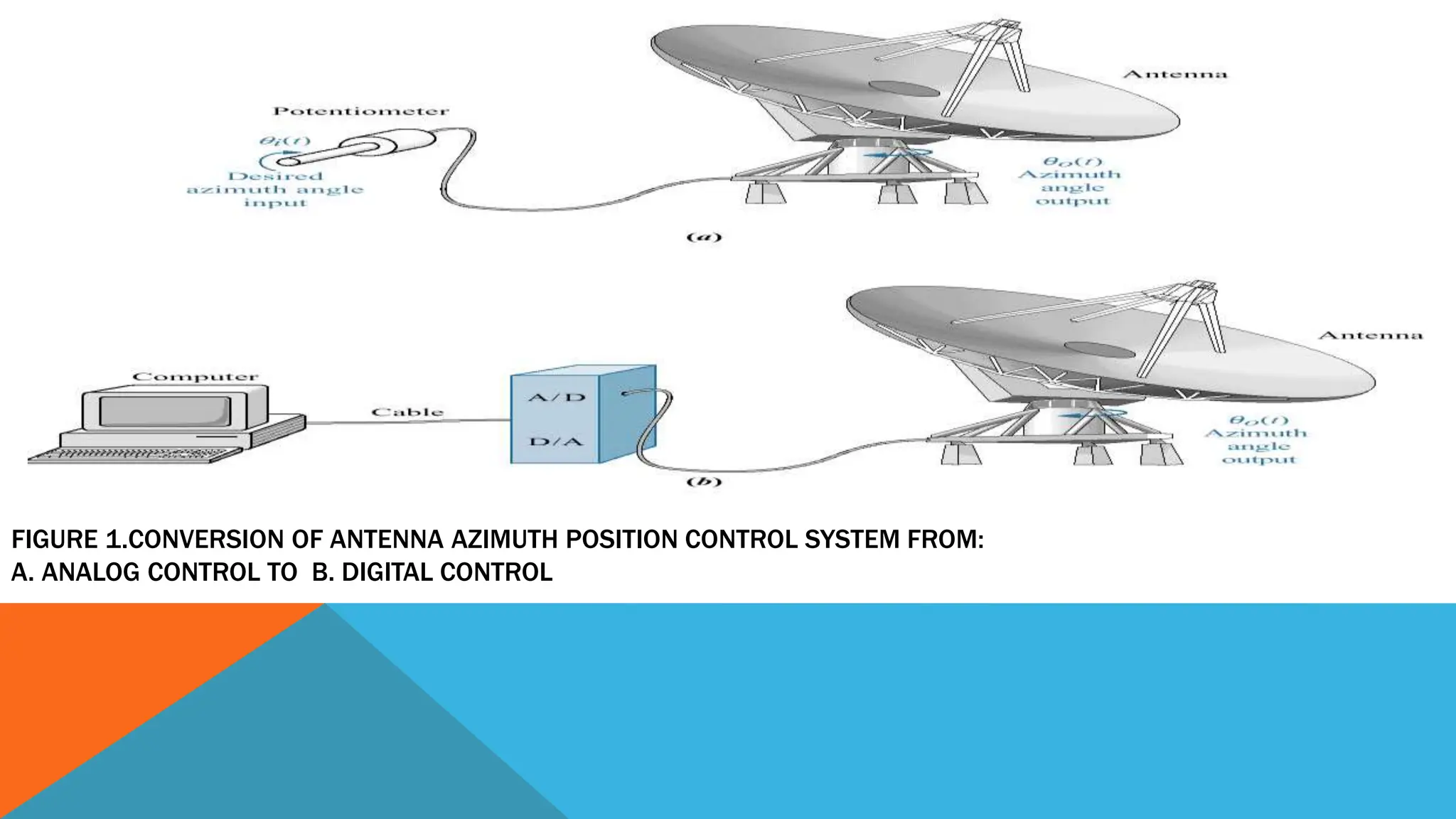
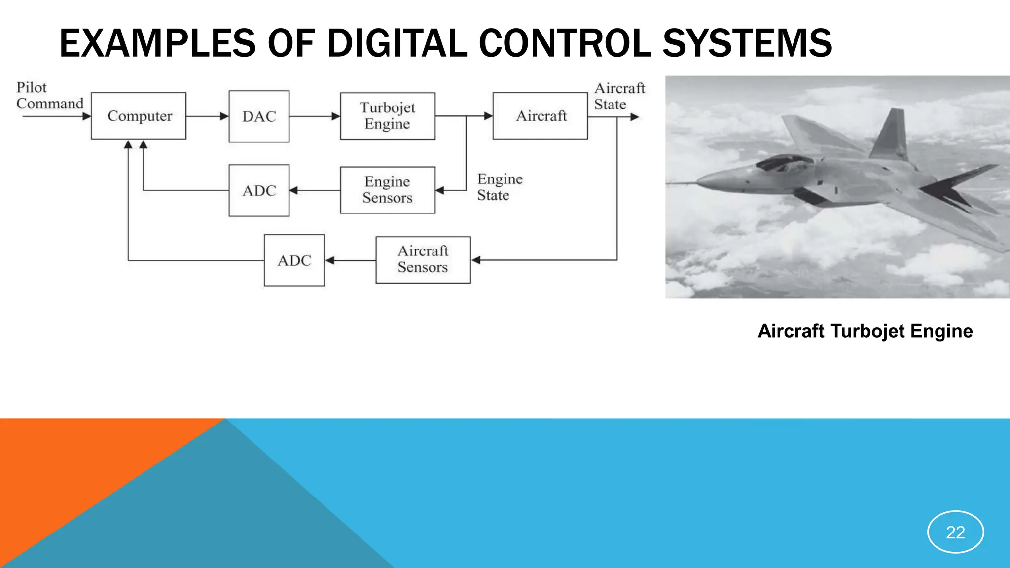
Applications in various industries include automotive speed regulators, autopilots in aviation, and robotics for trajectory control.
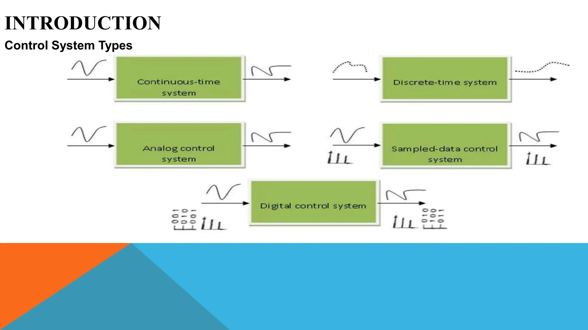
Different types of models for dynamic systems are described, such as physical, mathematical, analytical models, and their application in control systems.Different signal types such as continuous-time, discrete-time, sampled-data, and digital signals related to control systems are defined.
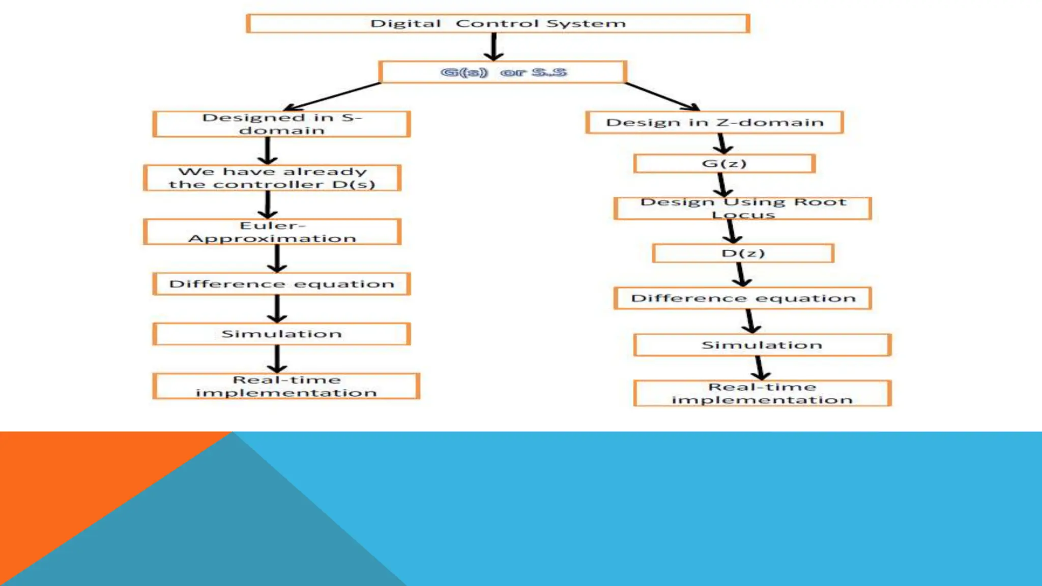
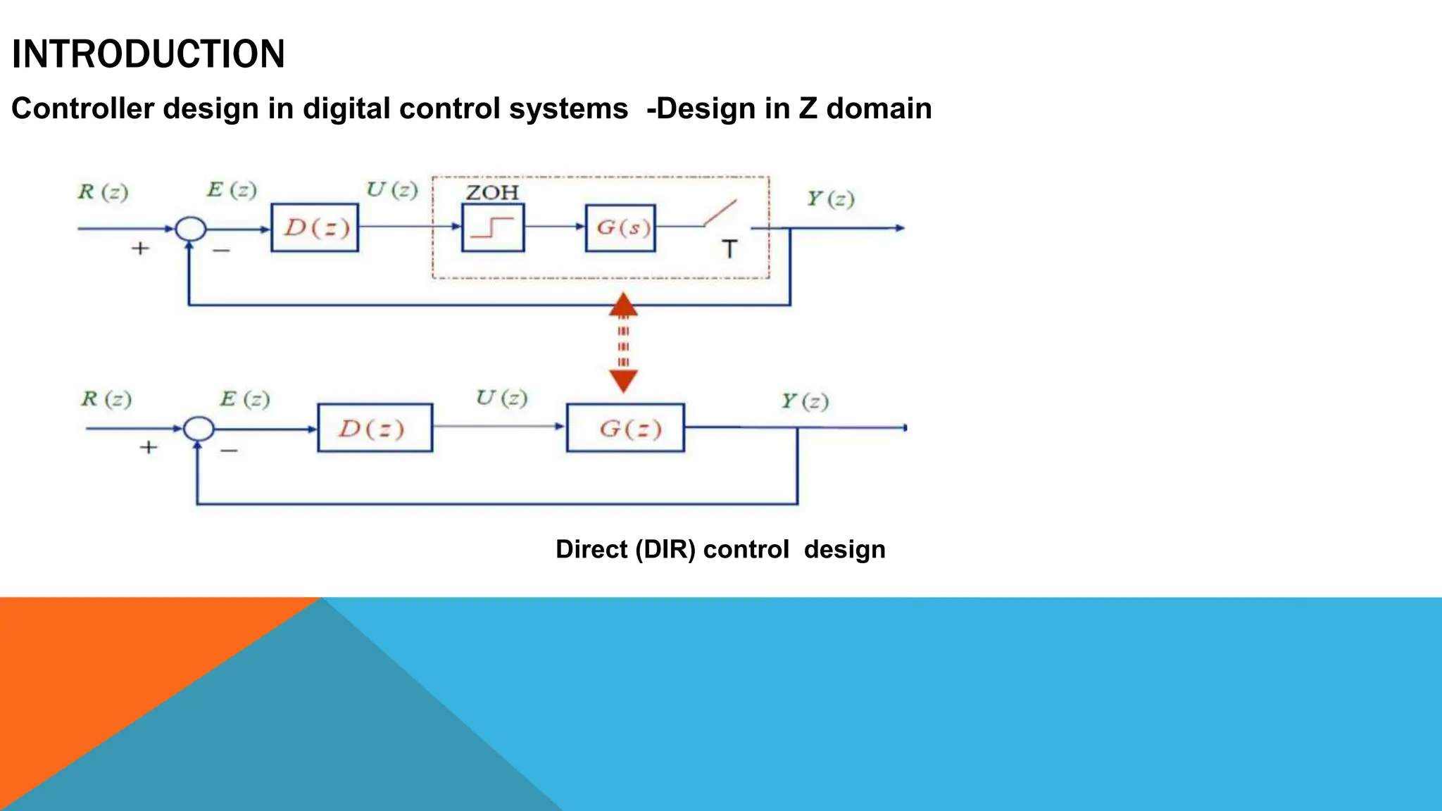
Overview of different control system types, with a particular focus on controller design in the digital domain, including digitization techniques.Methods for controller design, including use of difference equations, focusing on practical implementation using software like MATLAB.
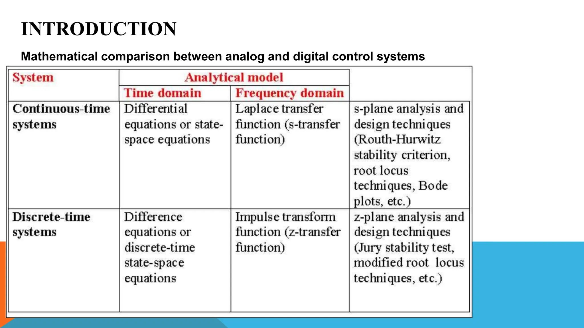
A mathematical comparison between analog and digital control systems, covering differential and difference equations, including examples.
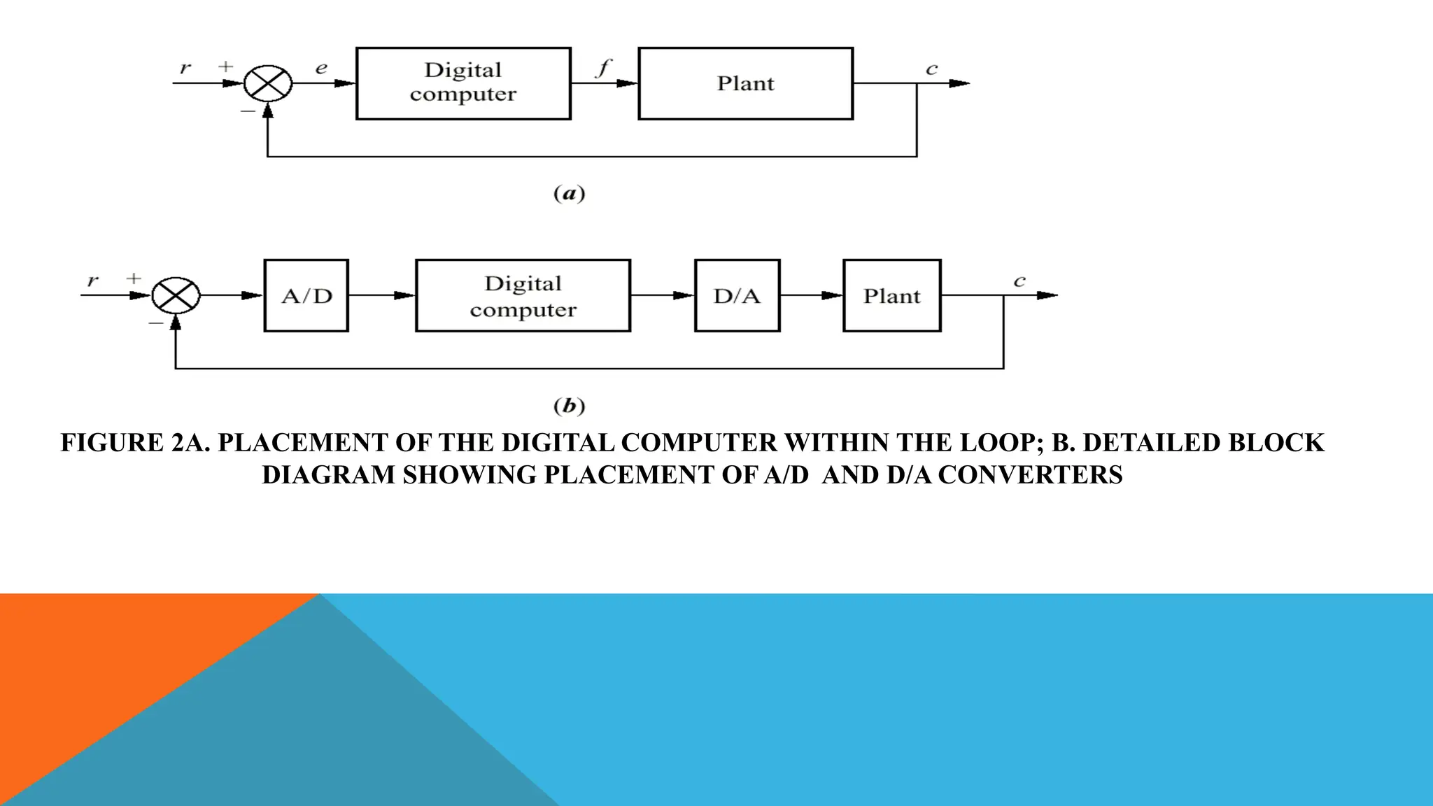
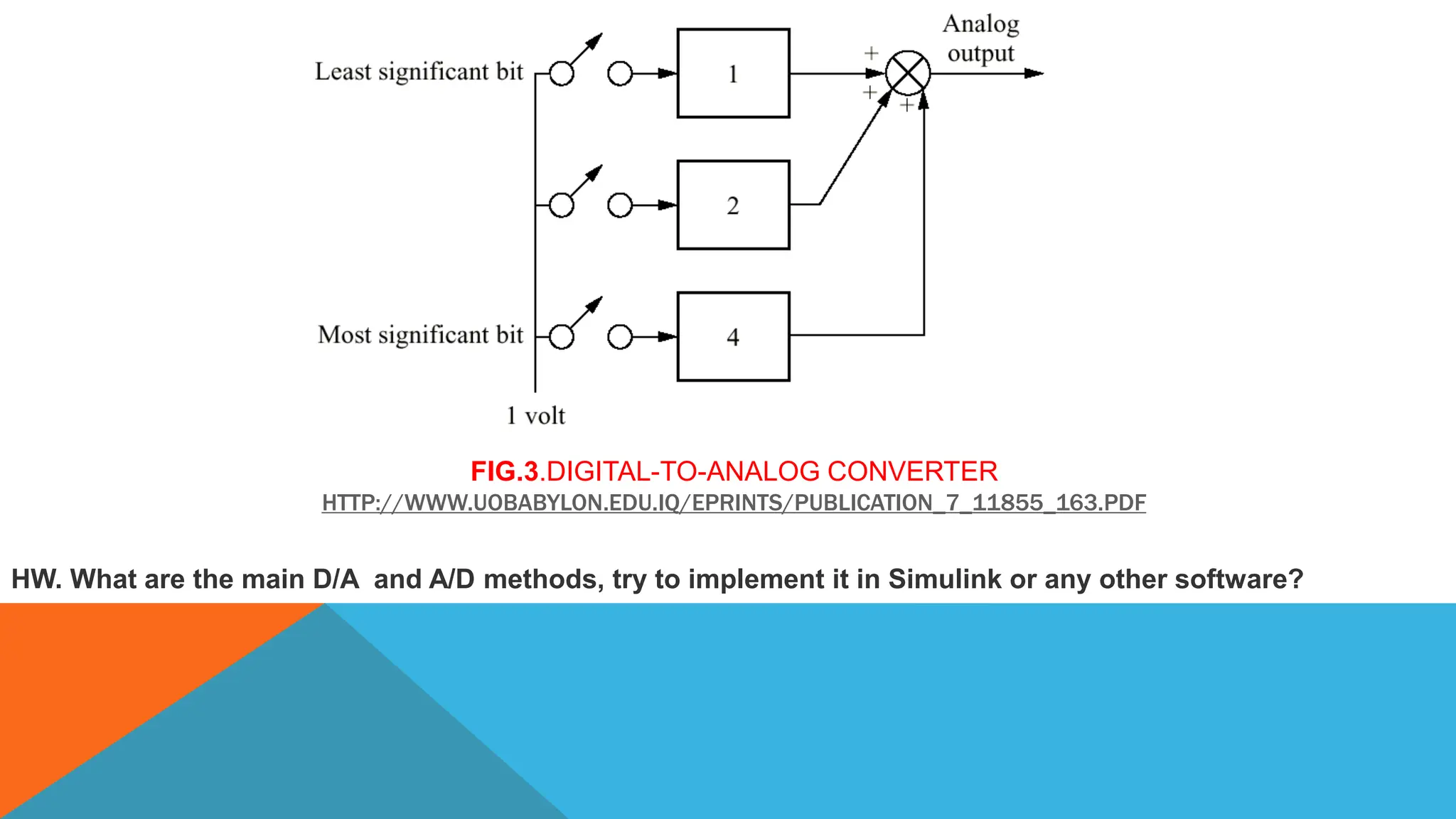
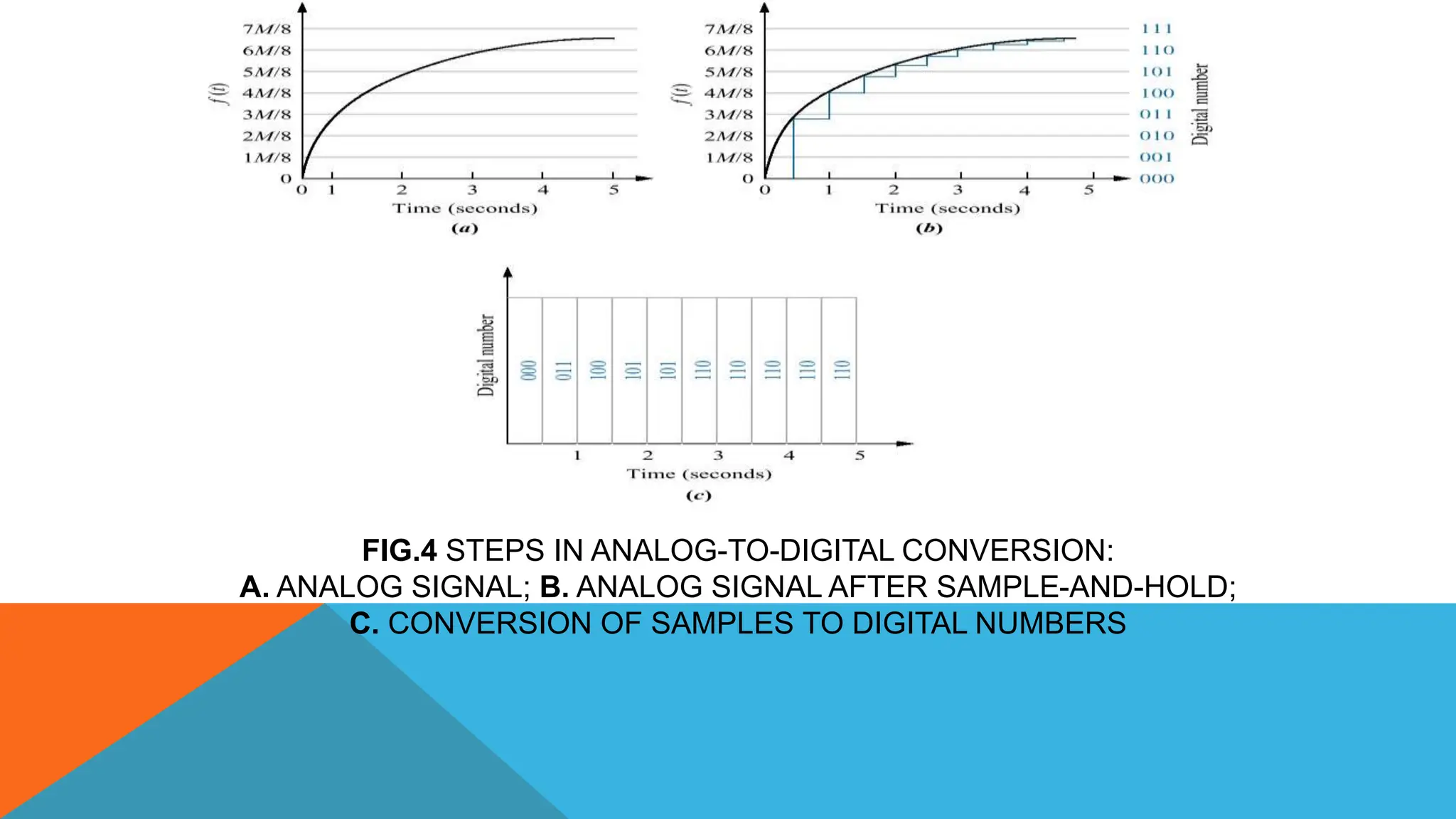
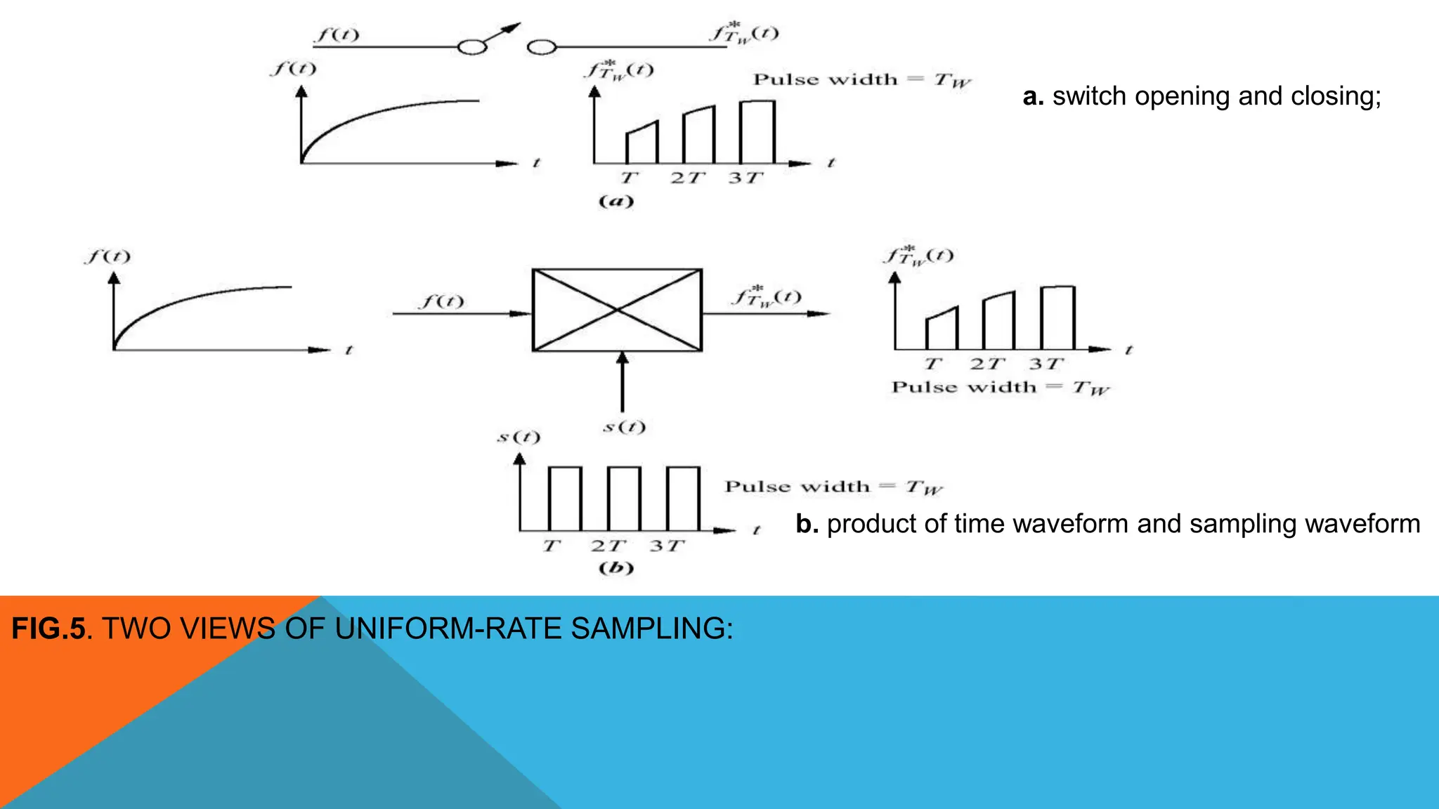
Integration of digital components in control systems using A/D and D/A converters, with examples of sampling and hold techniques.
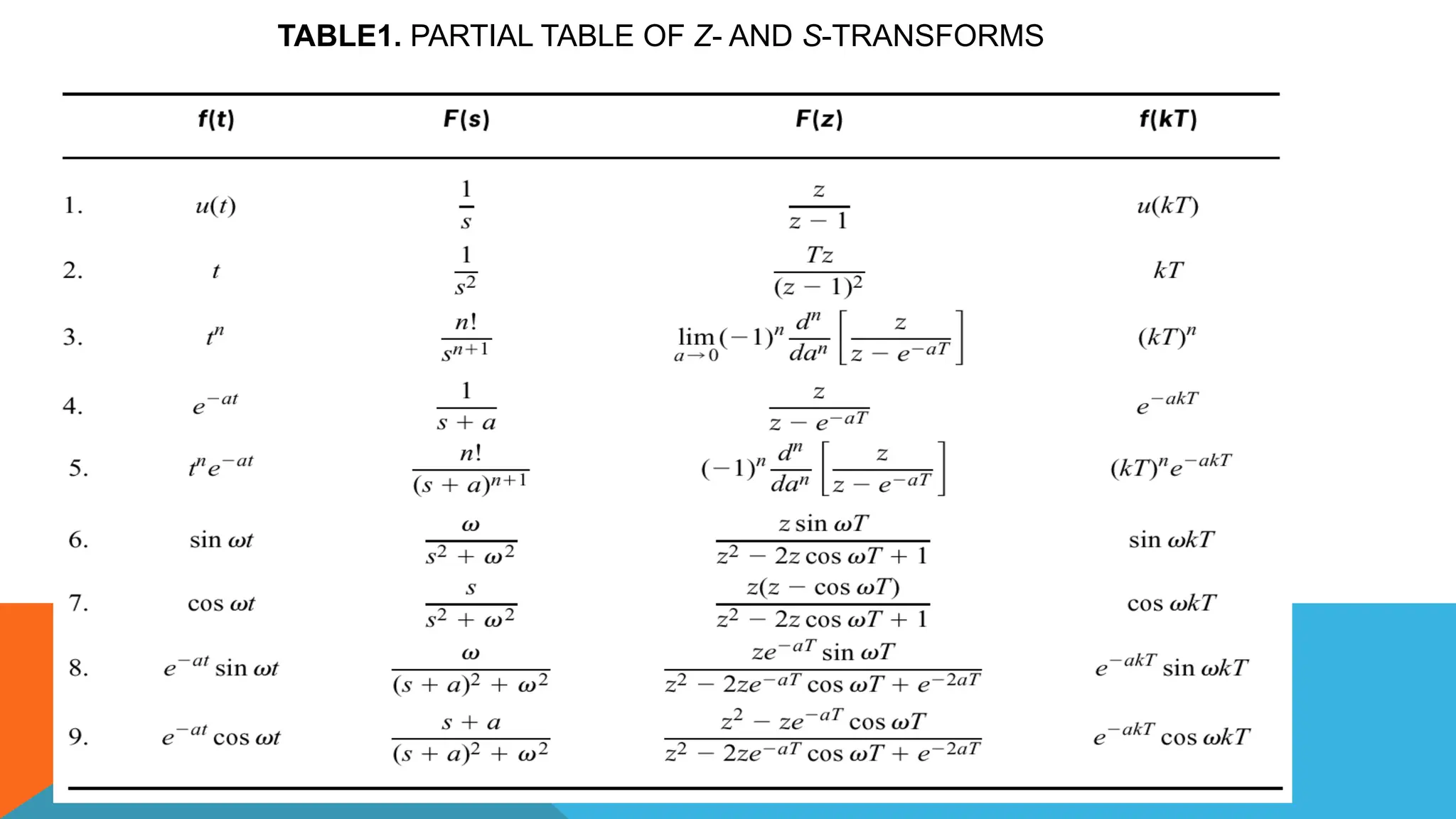
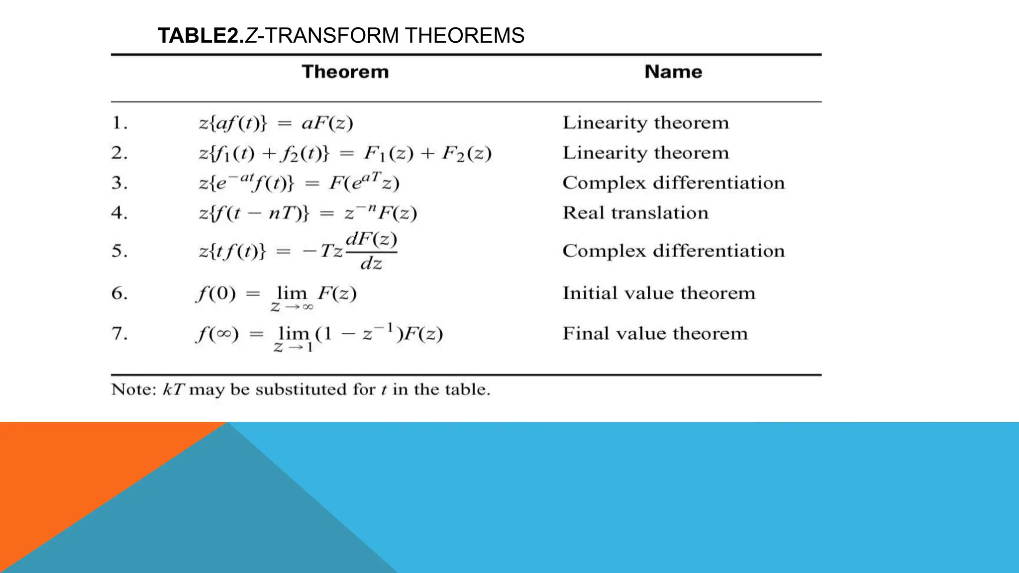
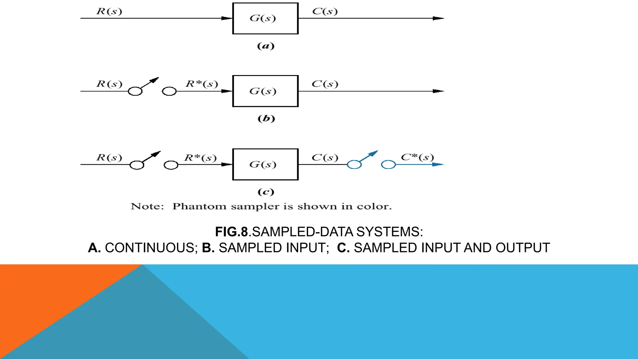
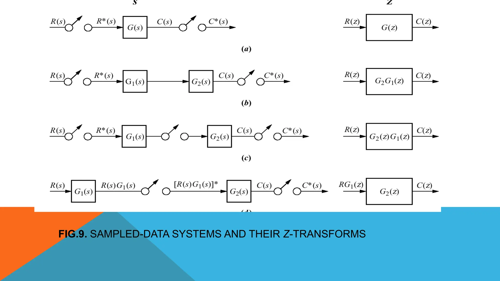
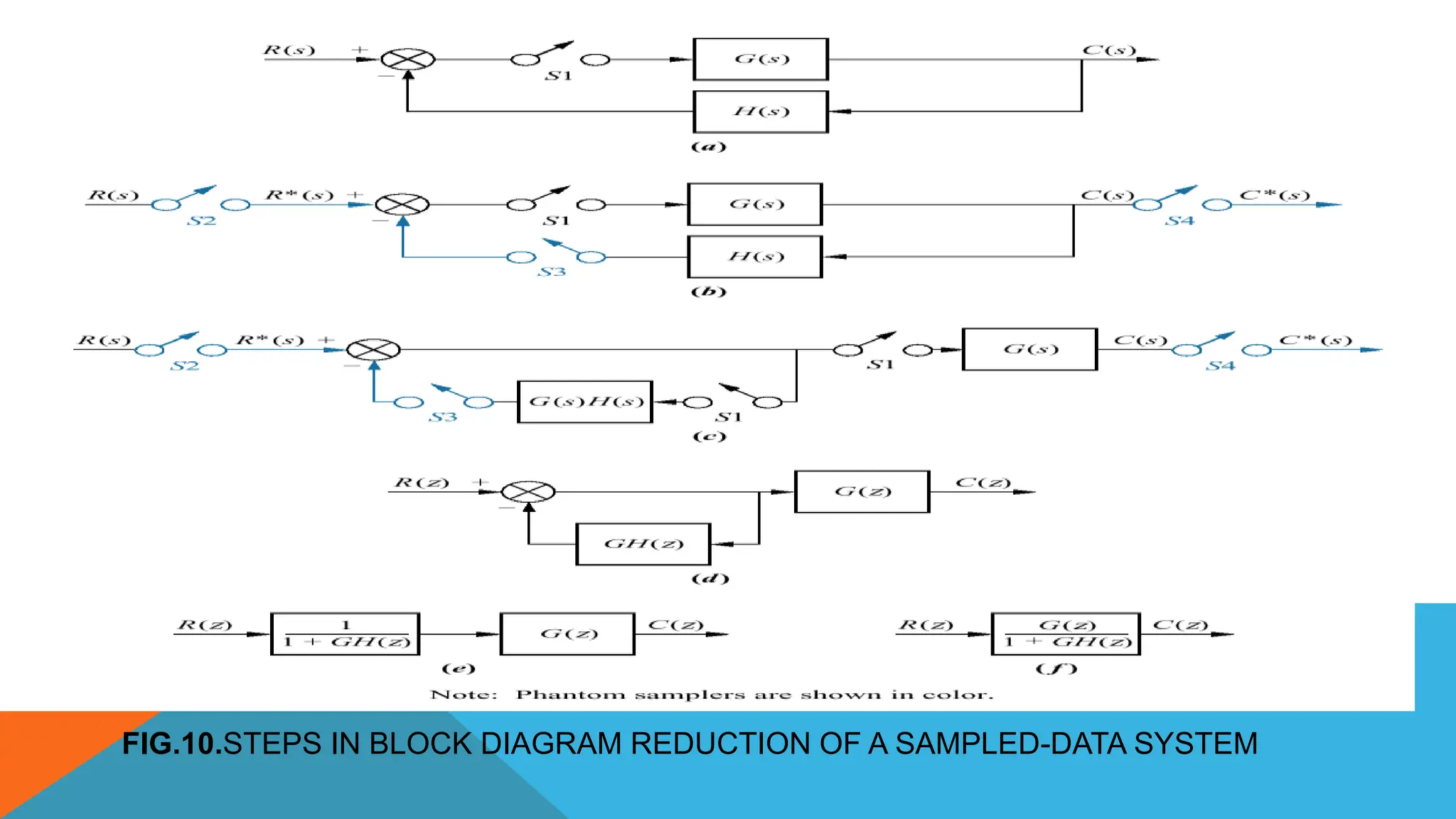
Tables and figures illustrating Z-transforms, sampled-data systems, and methods for block diagram reduction in sampled-data systems.
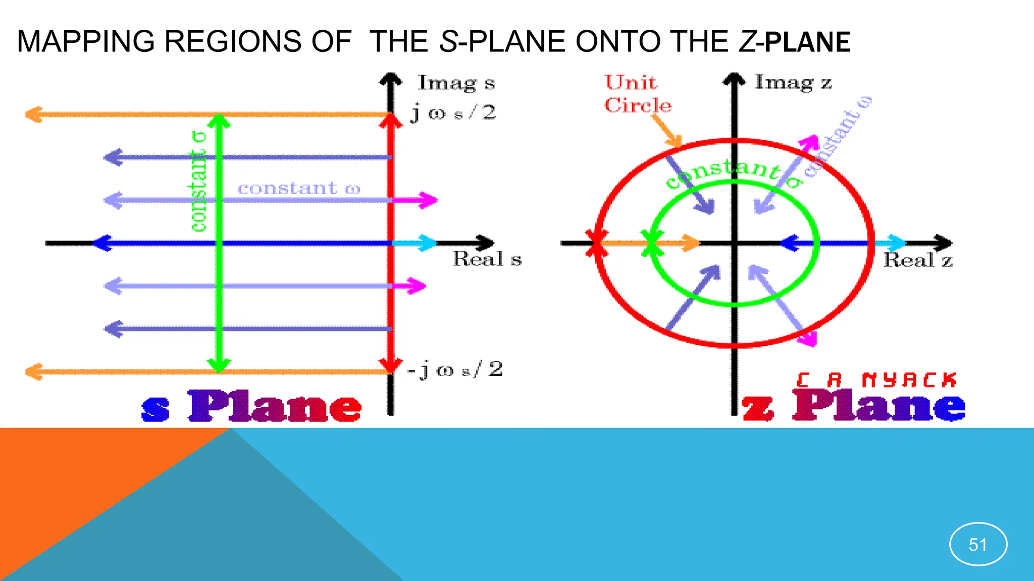
Steps in conformal mapping from S-plane to Z-plane, detailing various cases such as real and imaginary poles impacting stability.
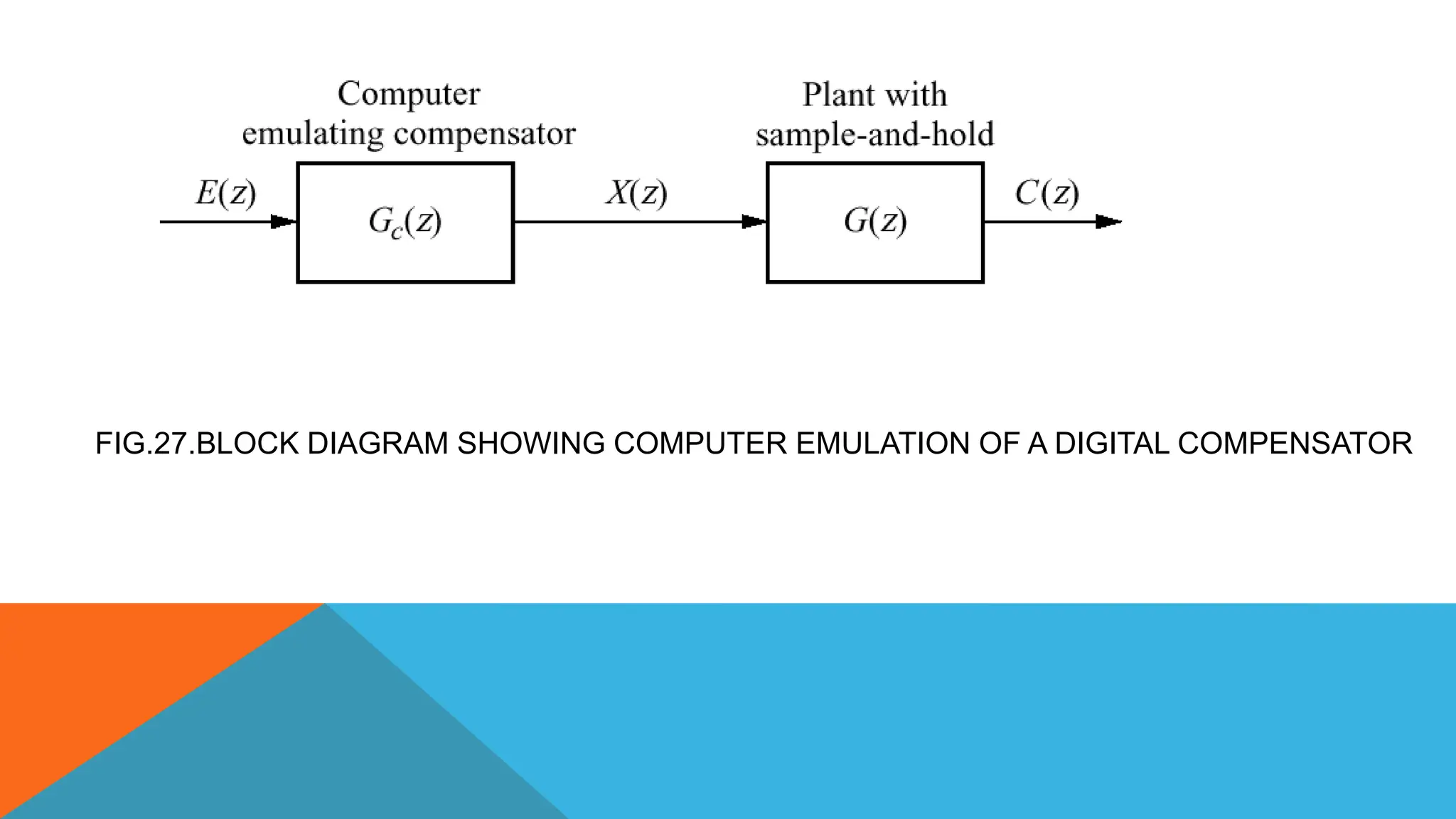
Illustration of complex systems such as missile control, compensation methods within digital frameworks, and system emulation.Fundamental discrete-time signal operations and applications, including professional projects related to digital control systems.
Closing remarks and gratitude for attendance, summarizing the importance of digital control systems in engineering.
DIGITAL CONTROL SYSTEMS
LECTURENO.1
PROF. DR. KHALAF S GAEID
ELECTRICAL ENGINEERING DEPARTMENT/ TIKRIT
UNIVERSITY
GAEIDKHALAF@GMAIL.COM
2.
1. A controlsystem consisting of interconnected components is designed to achieve a desired
purpose.
2. Modern control engineering practice includes the use of control design strategies for
improving manufacturing processes, the efficiency of energy use, advanced automobile
control, including rapid transit, among others.
3. We also discuss the notion of a design gap. The gap exists between the complex physical
system under investigation and the model used in the control system synthesis.
4. The iterative nature of design allows us to handle the design gap effectively while
accomplishing necessary tradeoffs in complexity, performance, and cost in order to meet
the design specifications.
Introduction to Control Systems Objectives
3.
Introduction
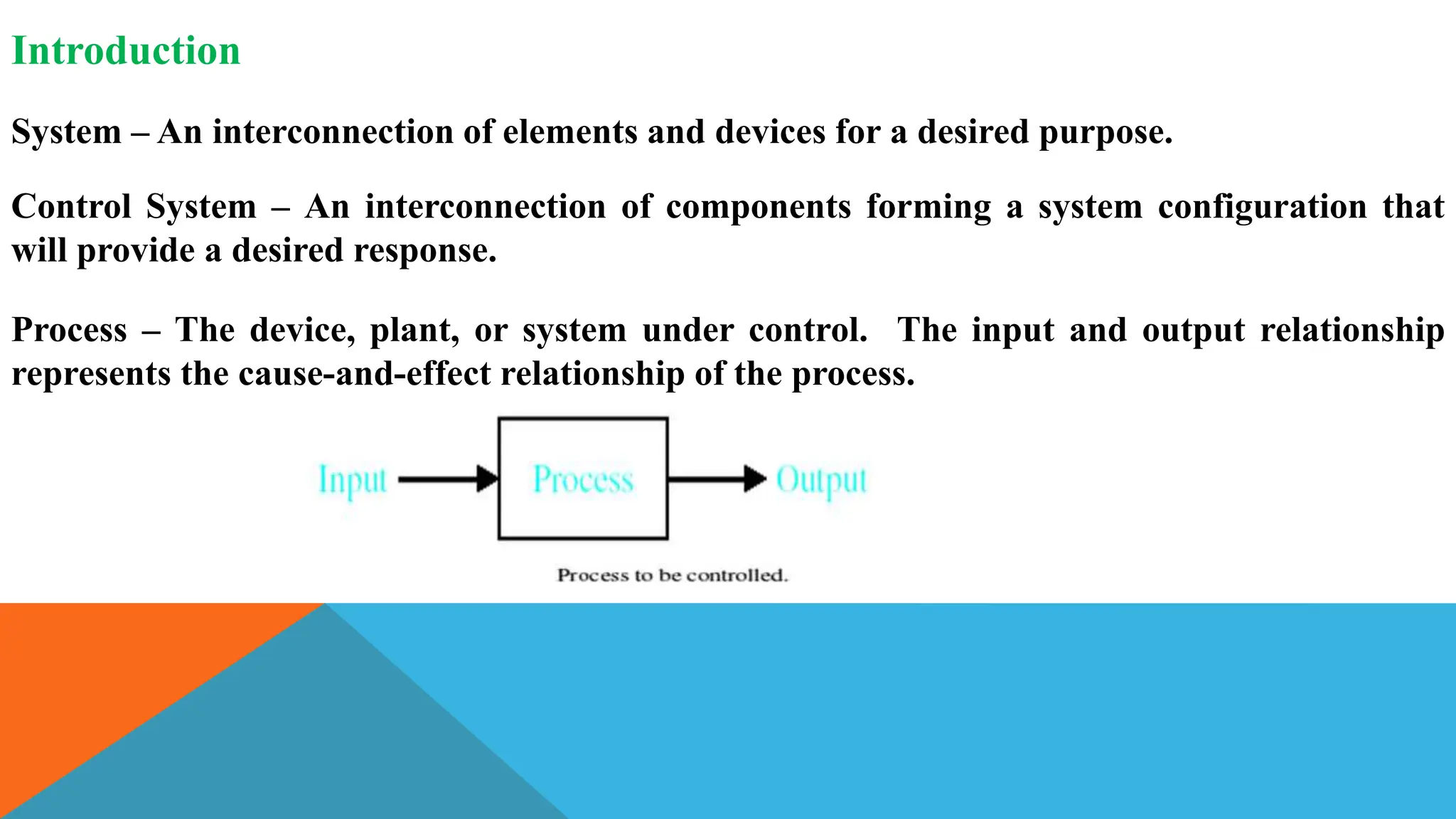
System – Aninterconnection of elements and devices for a desired purpose.
Control System – An interconnection of components forming a system configuration that
will provide a desired response.
Process – The device, plant, or system under control. The input and output relationship
represents the cause-and-effect relationship of the process.
4.
What is DigitalControl?
Automatic control is the science that develops techniques to steer, guide, control dynamic
systems.
These systems are built by humans and must perform a specific task. Examples of such
dynamic systems are found in biology, physics, robotics, finance, etc.
Digital Control means that the control laws are implemented in a digital device, such as a
microcontroller or a microprocessor. Such devices are light, fast and economical.
Digital Control Systems z-Plane Analysis of Discrete Time Control Systems
5.
INTRODUCTION
Digital control offersdistinct advantages over analog control that explain its
popularity.
Accuracy: Digital signals are more accurate than their analogue counterparts.
Implementation Errors: Implementation errors are negligible.
Flexibility: Modification of a digital controller is possible without complete
replacement.
Speed: Digital computers may yield superior performance at very fast speeds
Cost: Digital controllers are more economical than analogue controllers.
5
6.
DISADVANTAGES OF DIGITALCOMPUTERS
FROM THE TRACKING PERFORMANCE SIDE, THE ANALOG CONTROL SYSTEM
EXHIBITS GOOD PERFORMANCES THAN DIGITAL CONTROL SYSTEM.
DIGITAL CONTROL SYSTEM WILL INTRODUCE A DELAY IN THE LOOP.
6
https://www.mathworks.com/academia/books/search.html?q=digital%20control&
page=1
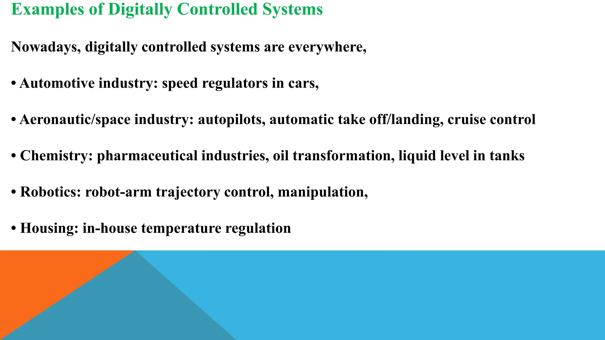
Examples of DigitallyControlled Systems
Nowadays, digitally controlled systems are everywhere,
• Automotive industry: speed regulators in cars,
• Aeronautic/space industry: autopilots, automatic take off/landing, cruise control
• Chemistry: pharmaceutical industries, oil transformation, liquid level in tanks
• Robotics: robot-arm trajectory control, manipulation,
• Housing: in-house temperature regulation
9.
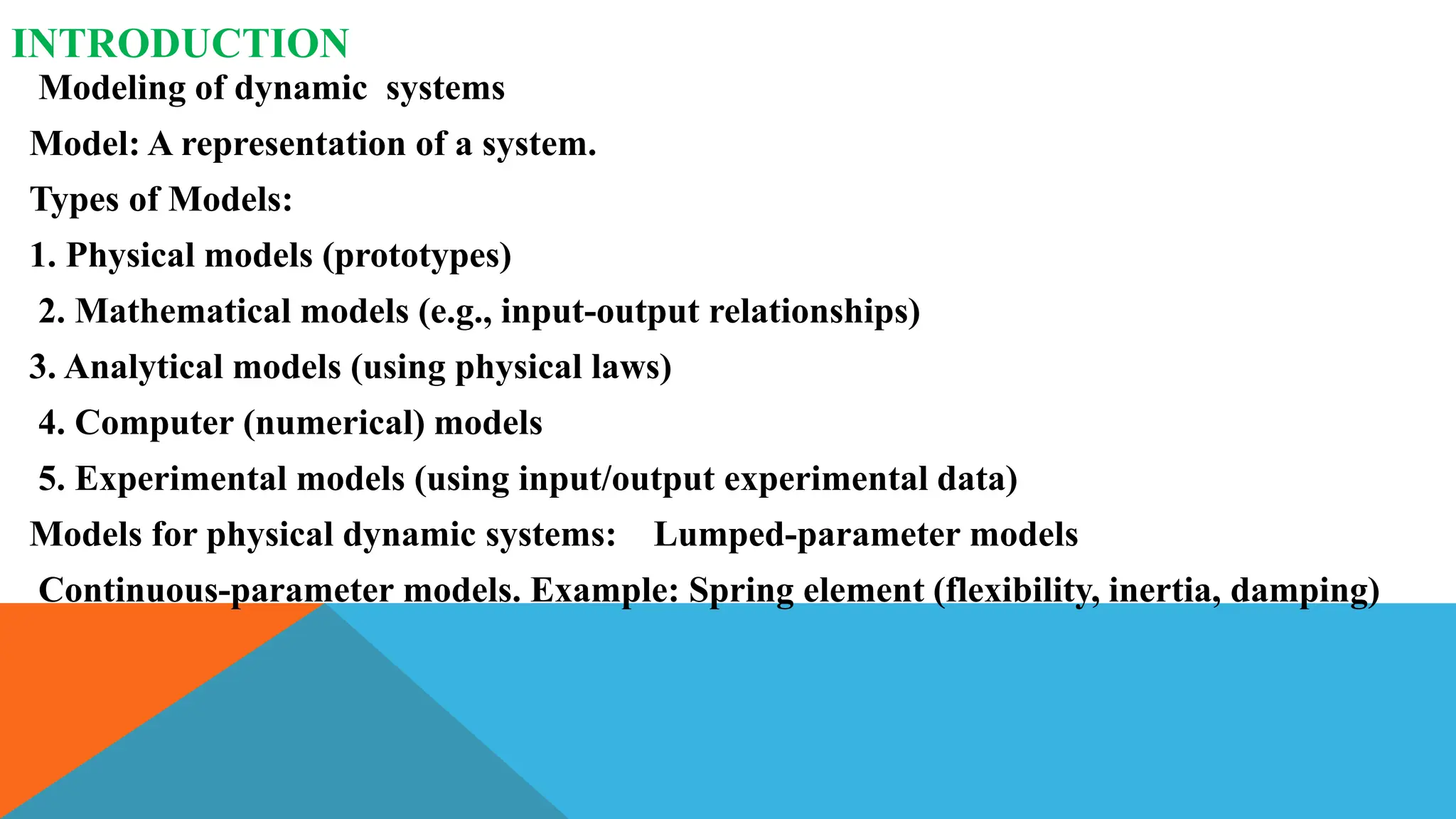
INTRODUCTION
Modeling of dynamicsystems
Model: A representation of a system.
Types of Models:
1. Physical models (prototypes)
2. Mathematical models (e.g., input-output relationships)
3. Analytical models (using physical laws)
4. Computer (numerical) models
5. Experimental models (using input/output experimental data)
Models for physical dynamic systems: Lumped-parameter models
Continuous-parameter models. Example: Spring element (flexibility, inertia, damping)
10.
INTRODUCTION
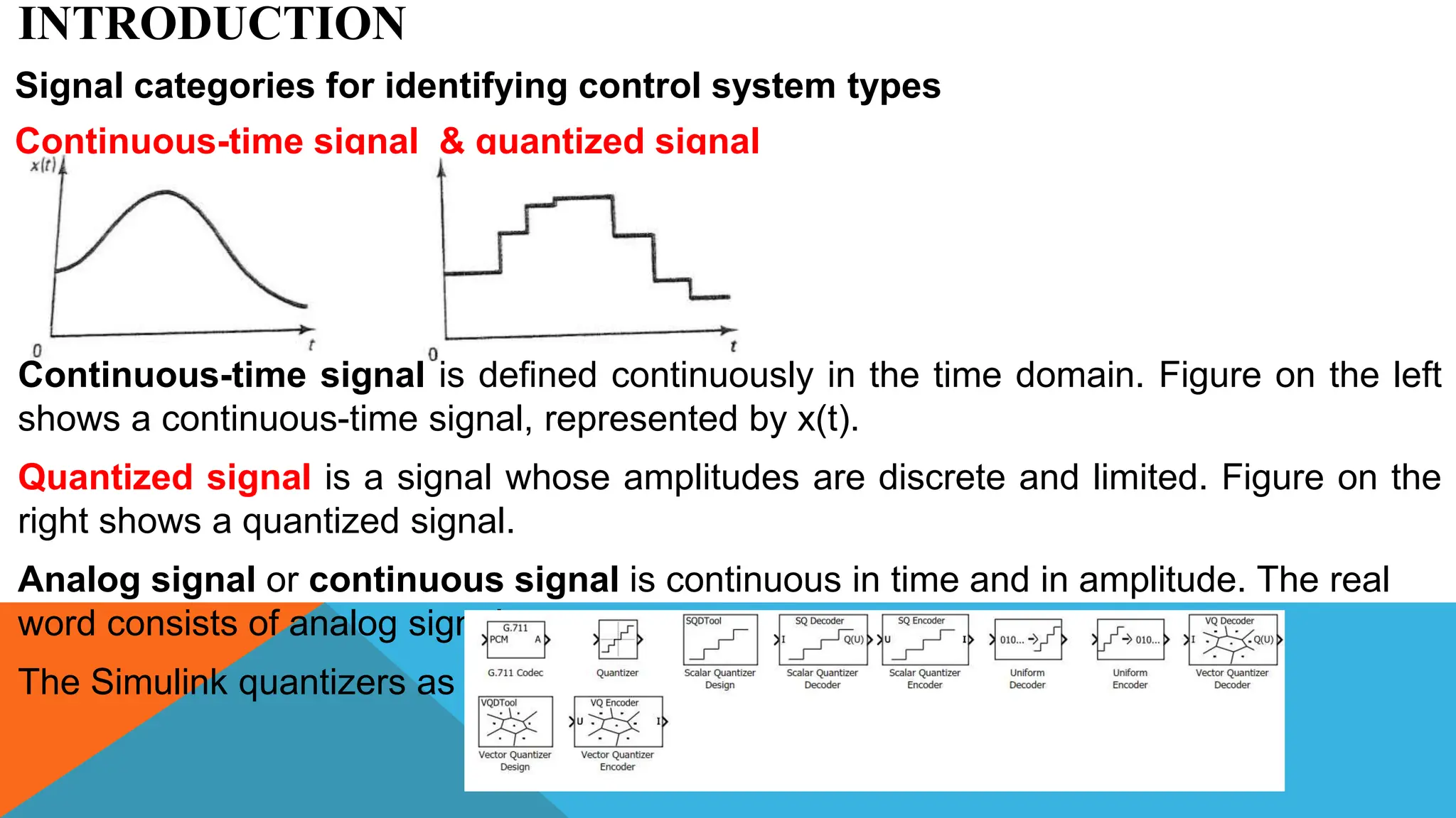
Signal categories foridentifying control system types
Continuous-time signal & quantized signal
Continuous-time signal is defined continuously in the time domain. Figure on the left
shows a continuous-time signal, represented by x(t).
Quantized signal is a signal whose amplitudes are discrete and limited. Figure on the
right shows a quantized signal.
Analog signal or continuous signal is continuous in time and in amplitude. The real
word consists of analog signals.
The Simulink quantizers as
11.
INTRODUCTION
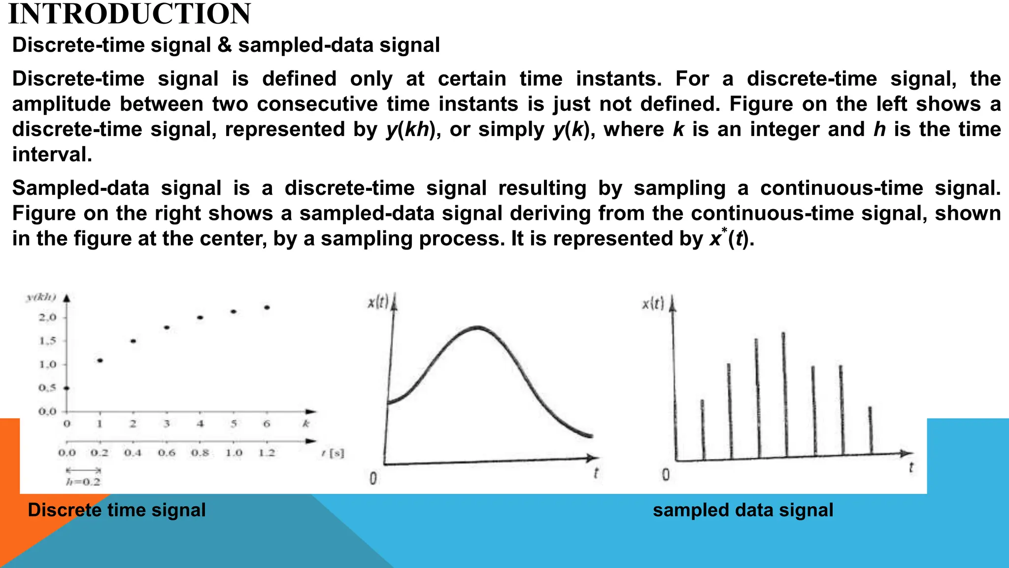
Discrete-time signal &sampled-data signal
Discrete-time signal is defined only at certain time instants. For a discrete-time signal, the
amplitude between two consecutive time instants is just not defined. Figure on the left shows a
discrete-time signal, represented by y(kh), or simply y(k), where k is an integer and h is the time
interval.
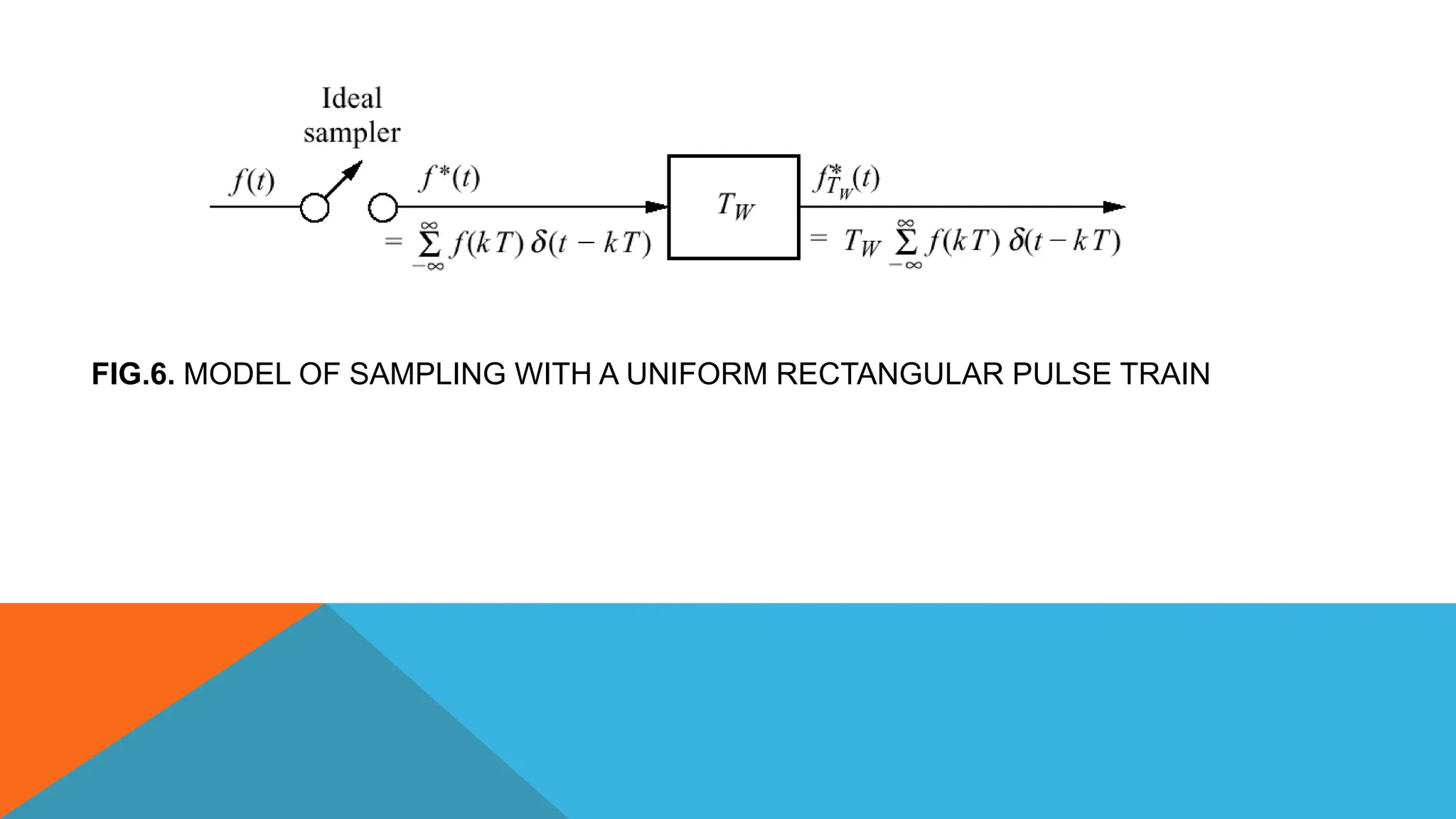
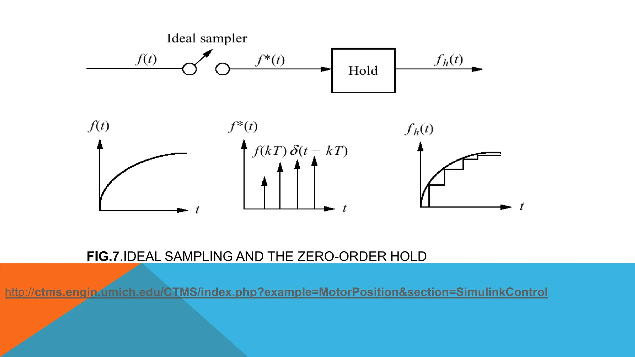
Sampled-data signal is a discrete-time signal resulting by sampling a continuous-time signal.
Figure on the right shows a sampled-data signal deriving from the continuous-time signal, shown
in the figure at the center, by a sampling process. It is represented by x
∗
(t).
Discrete time signal sampled data signal
12.
INTRODUCTION
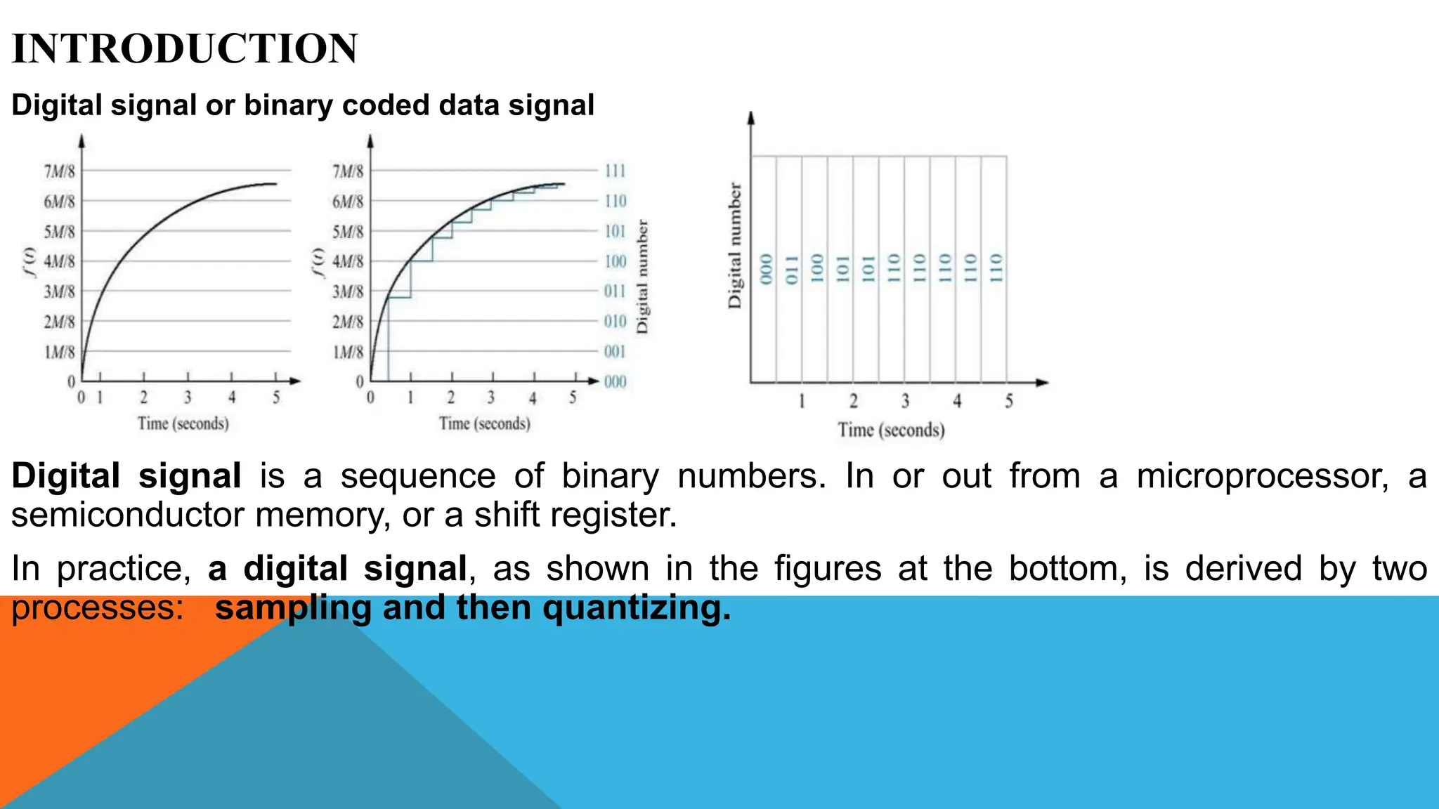
Digital signal orbinary coded data signal
Digital signal is a sequence of binary numbers. In or out from a microprocessor, a
semiconductor memory, or a shift register.
In practice, a digital signal, as shown in the figures at the bottom, is derived by two
processes: sampling and then quantizing.
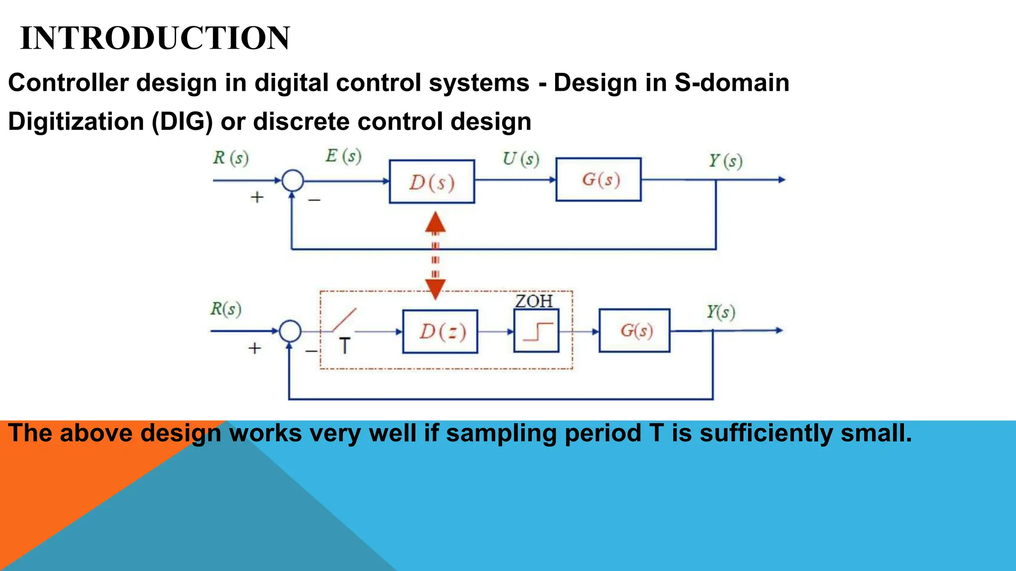
INTRODUCTION
Controller design indigital control systems - Design in S-domain
Digitization (DIG) or discrete control design
The above design works very well if sampling period T is sufficiently small.
16.
INTRODUCTION
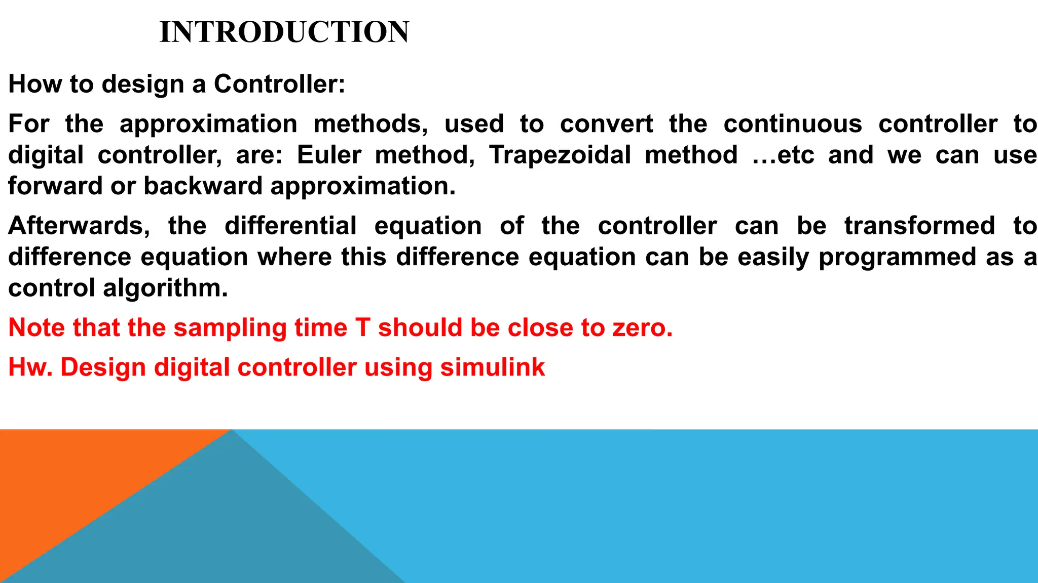
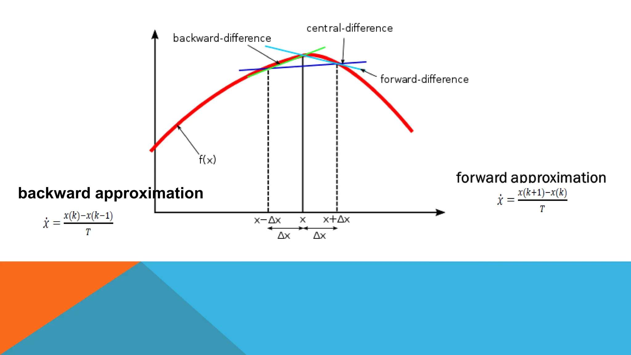
How to designa Controller:
For the approximation methods, used to convert the continuous controller to
digital controller, are: Euler method, Trapezoidal method …etc and we can use
forward or backward approximation.
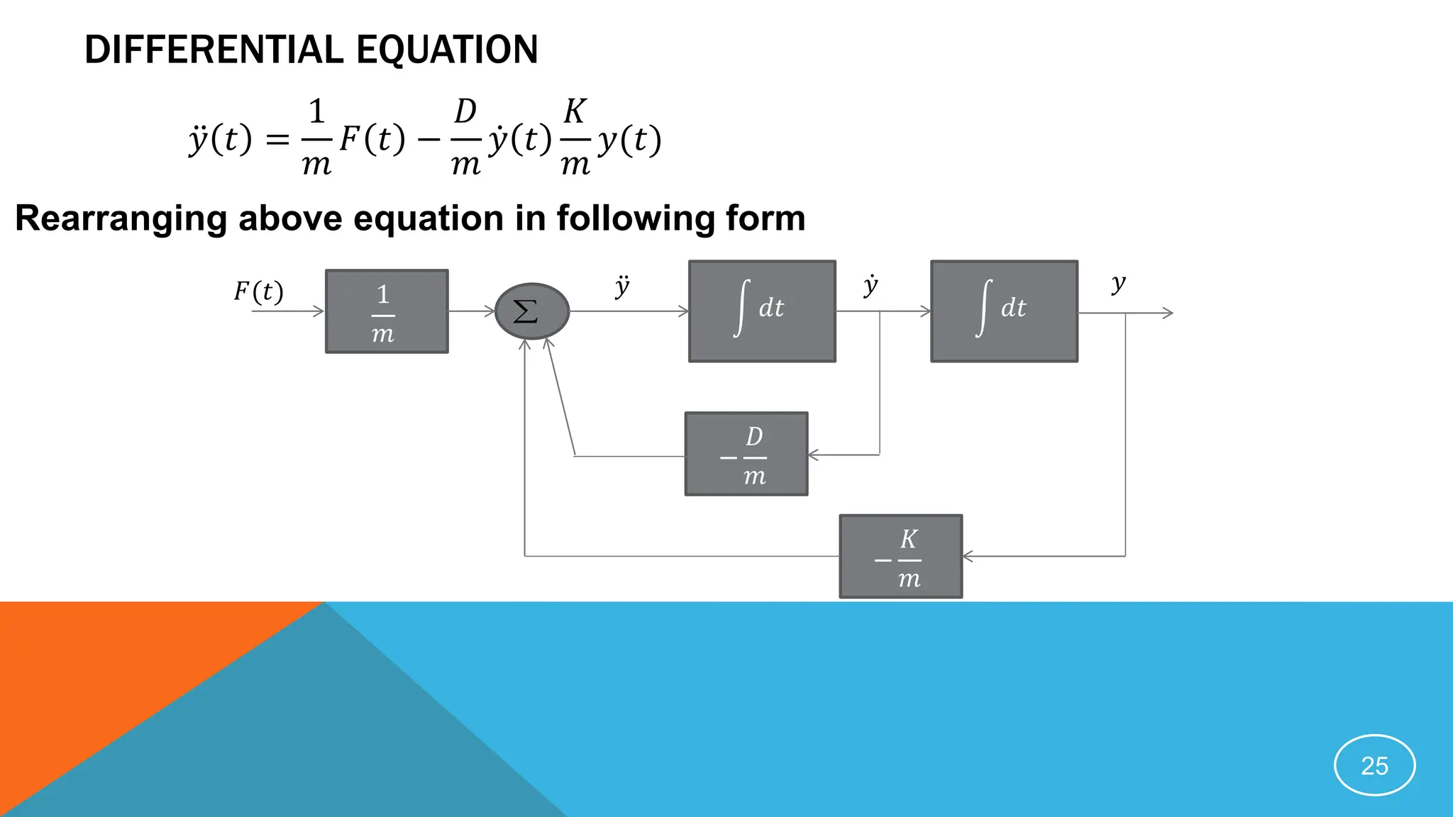
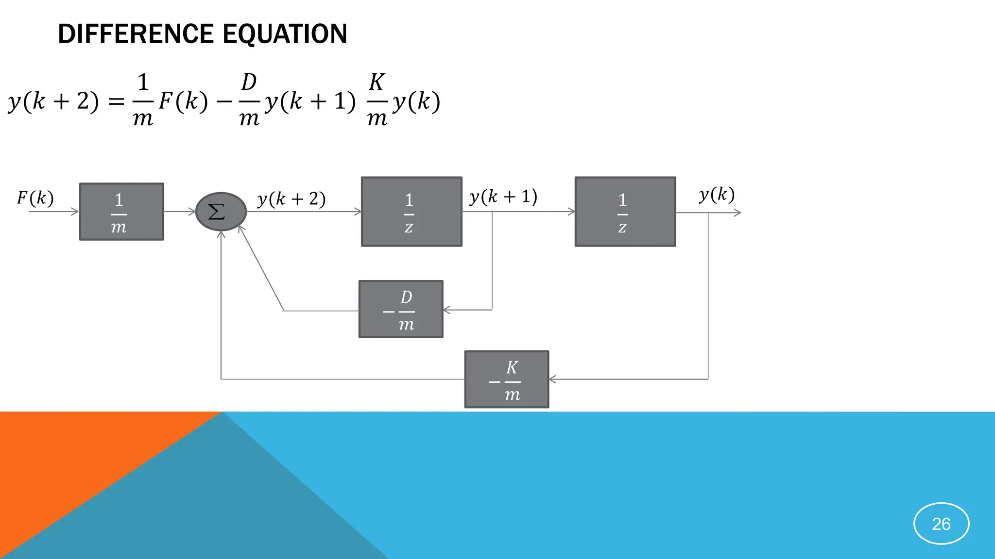
Afterwards, the differential equation of the controller can be transformed to
difference equation where this difference equation can be easily programmed as a
control algorithm.
Note that the sampling time T should be close to zero.
Hw. Design digital controller using simulink
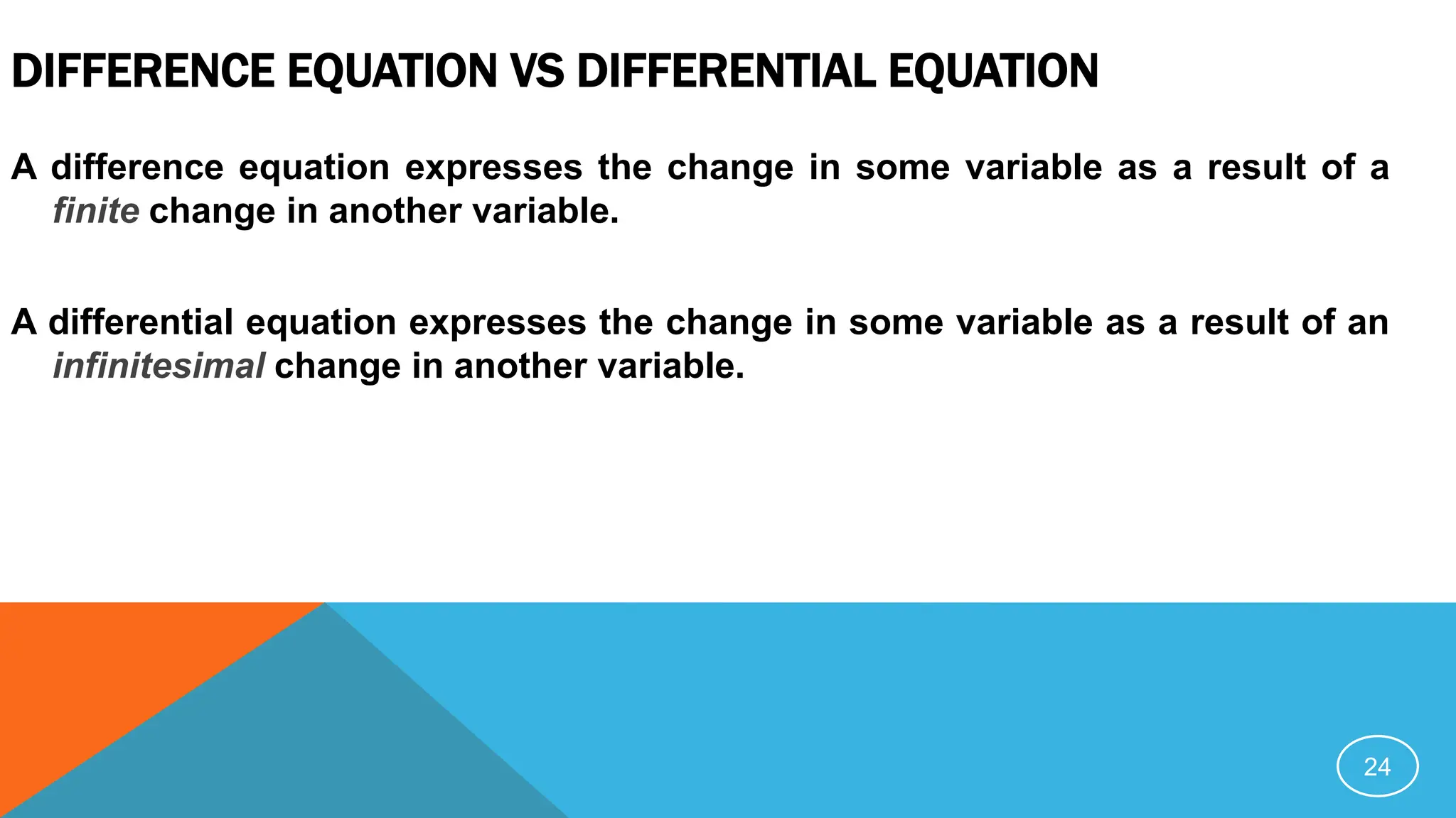
DIFFERENCE EQUATION VSDIFFERENTIAL EQUATION
A difference equation expresses the change in some variable as a result of a
finite change in another variable.
A differential equation expresses the change in some variable as a result of an
infinitesimal change in another variable.
24
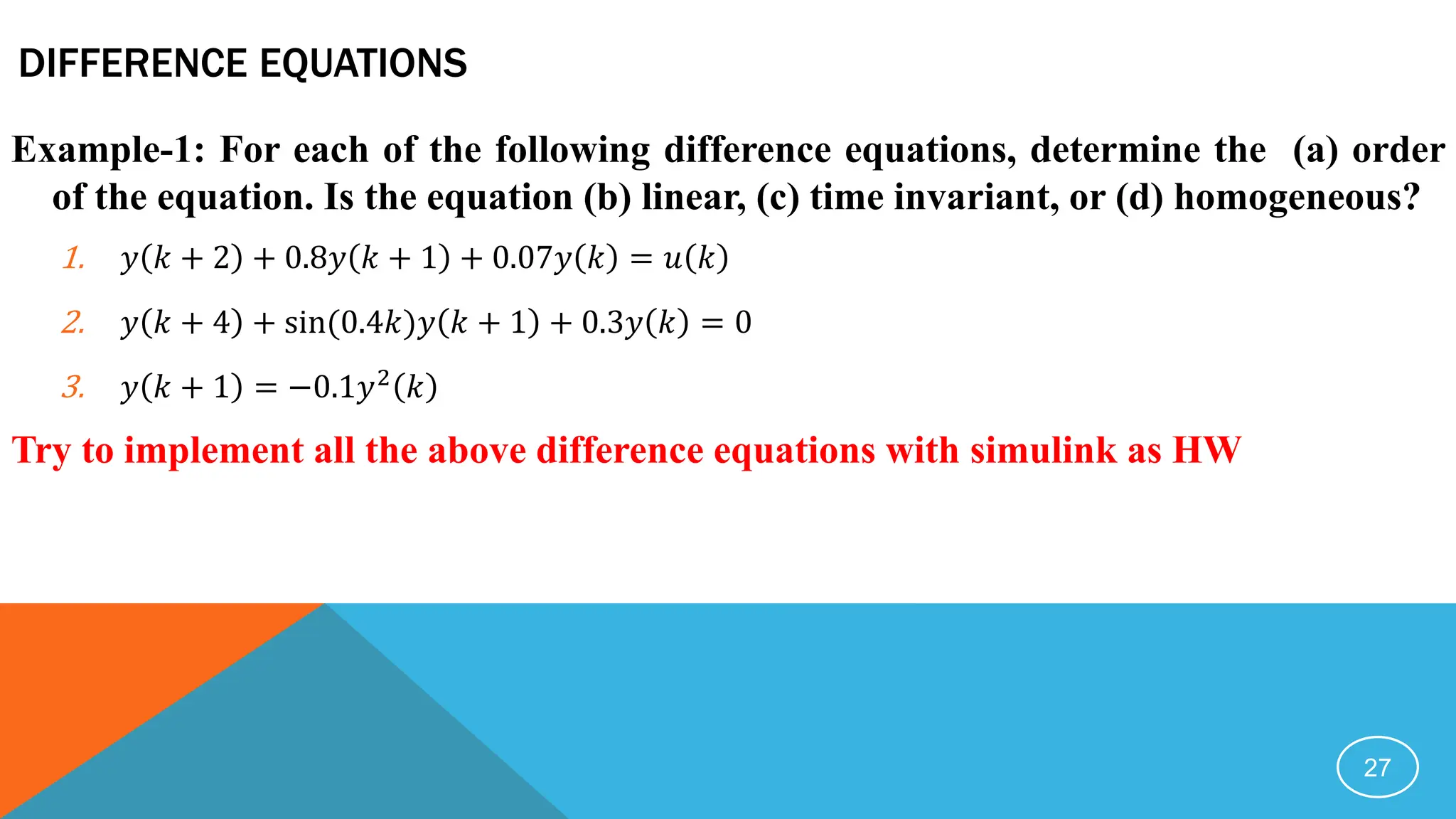
DIFFERENCE EQUATIONS
Example-1: Foreach of the following difference equations, determine the (a) order
of the equation. Is the equation (b) linear, (c) time invariant, or (d) homogeneous?
1. 𝑦 𝑘 + 2 + 0.8𝑦 𝑘 + 1 + 0.07𝑦 𝑘 = 𝑢 𝑘
2. 𝑦 𝑘 + 4 + sin(0.4𝑘)𝑦 𝑘 + 1 + 0.3𝑦 𝑘 = 0
3. 𝑦 𝑘 + 1 = −0.1𝑦2
𝑘
Try to implement all the above difference equations with simulink as HW
27
28.
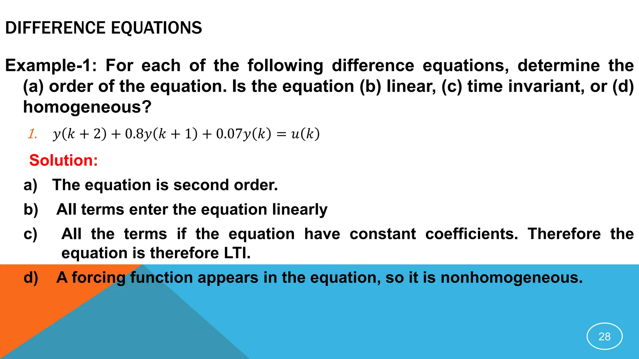
DIFFERENCE EQUATIONS
Example-1: Foreach of the following difference equations, determine the
(a) order of the equation. Is the equation (b) linear, (c) time invariant, or (d)
homogeneous?
1. 𝑦 𝑘 + 2 + 0.8𝑦 𝑘 + 1 + 0.07𝑦 𝑘 = 𝑢 𝑘
Solution:
a) The equation is second order.
b) All terms enter the equation linearly
c) All the terms if the equation have constant coefficients. Therefore the
equation is therefore LTI.
d) A forcing function appears in the equation, so it is nonhomogeneous.
28
29.
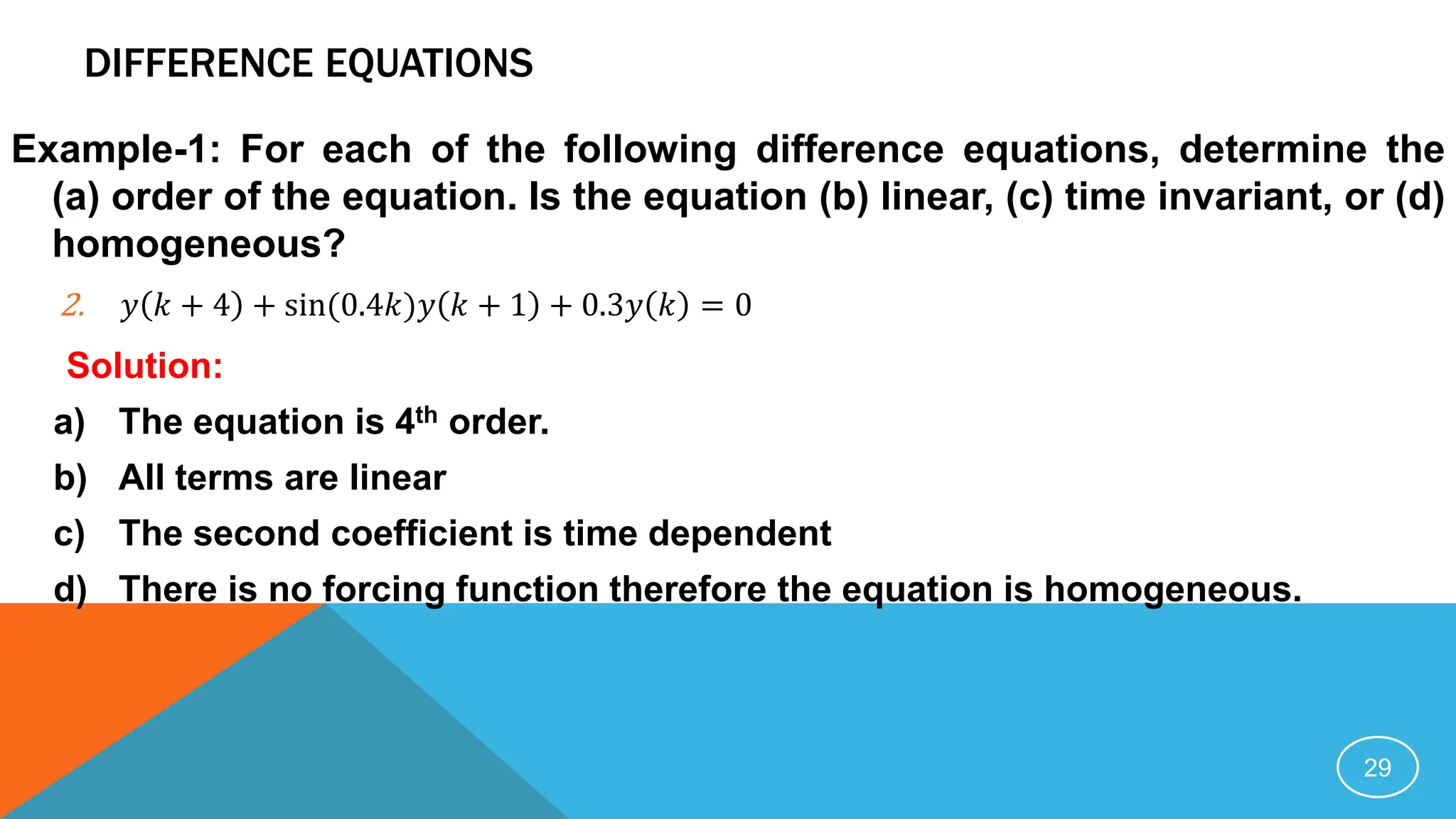
DIFFERENCE EQUATIONS
Example-1: Foreach of the following difference equations, determine the
(a) order of the equation. Is the equation (b) linear, (c) time invariant, or (d)
homogeneous?
2. 𝑦 𝑘 + 4 + sin(0.4𝑘)𝑦 𝑘 + 1 + 0.3𝑦 𝑘 = 0
Solution:
a) The equation is 4th order.
b) All terms are linear
c) The second coefficient is time dependent
d) There is no forcing function therefore the equation is homogeneous.
29
30.
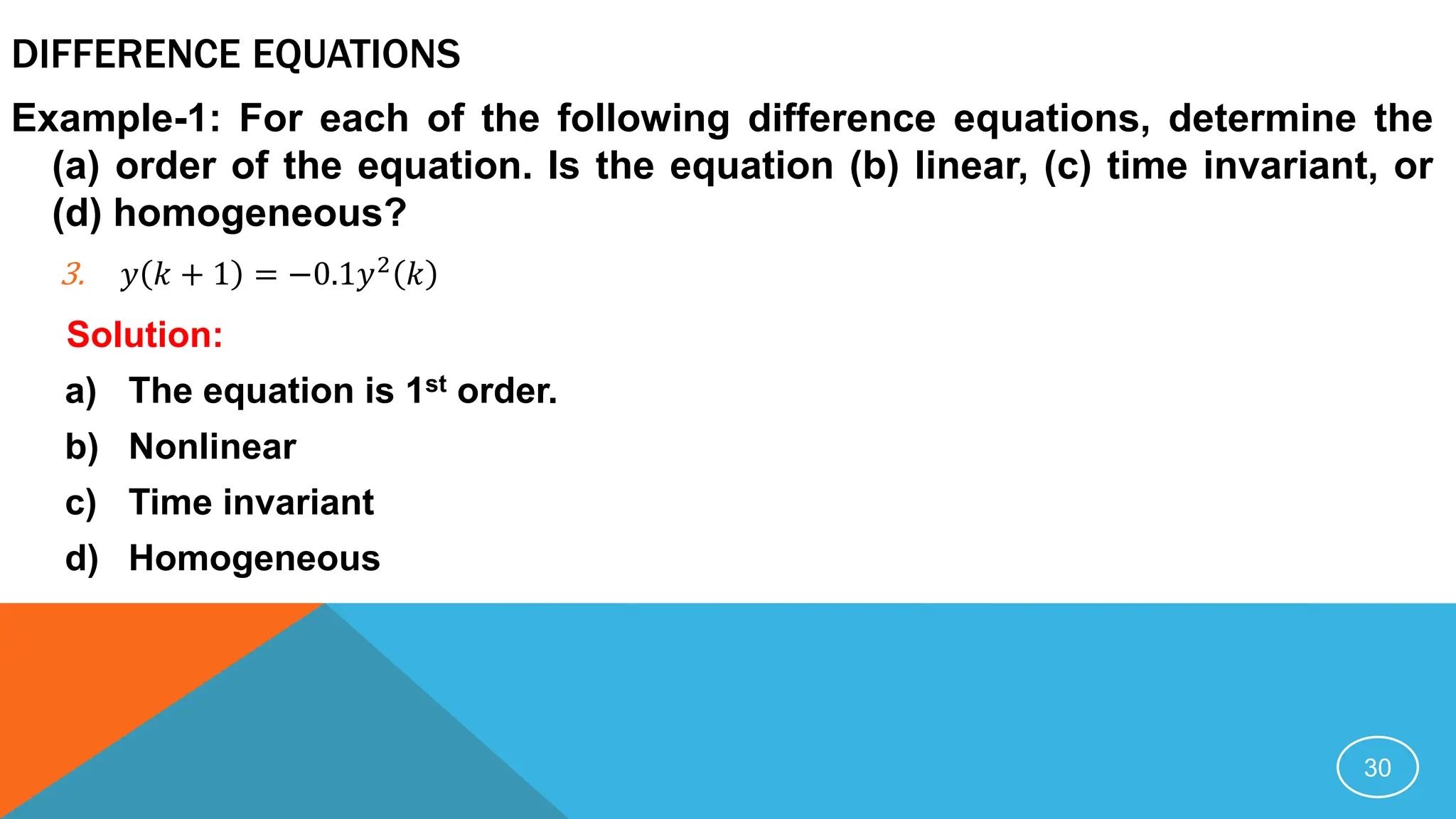
DIFFERENCE EQUATIONS
Example-1: Foreach of the following difference equations, determine the
(a) order of the equation. Is the equation (b) linear, (c) time invariant, or
(d) homogeneous?
3. 𝑦 𝑘 + 1 = −0.1𝑦2
𝑘
Solution:
a) The equation is 1st order.
b) Nonlinear
c) Time invariant
d) Homogeneous
30
31.
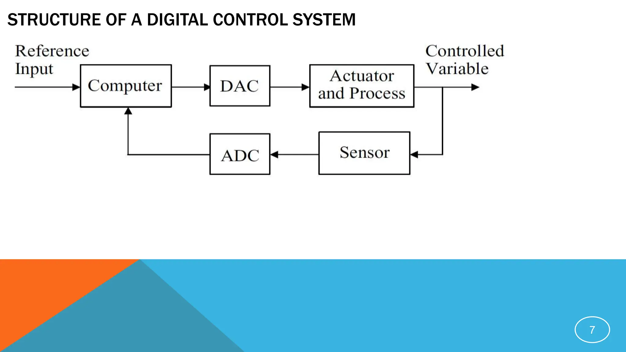
FIGURE 2A. PLACEMENTOF THE DIGITAL COMPUTER WITHIN THE LOOP; B. DETAILED BLOCK
DIAGRAM SHOWING PLACEMENT OF A/D AND D/A CONVERTERS
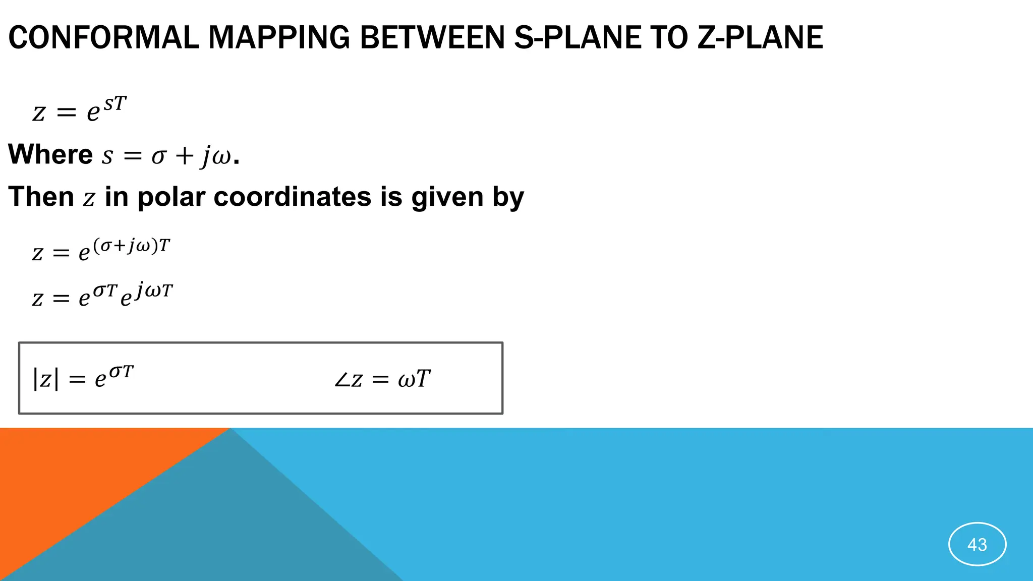
CONFORMAL MAPPING BETWEENS-PLANE TO Z-PLANE
Where 𝑠 = 𝜎 + 𝑗𝜔.
Then 𝑧 in polar coordinates is given by
43
𝑧 = 𝑒(𝜎+𝑗𝜔)𝑇
𝑧 = 𝑒𝜎𝑇
𝑒𝑗𝜔𝑇
∠𝑧 = 𝜔𝑇
𝑧 = 𝑒𝜎𝑇
𝑧 = 𝑒𝑠𝑇
44.
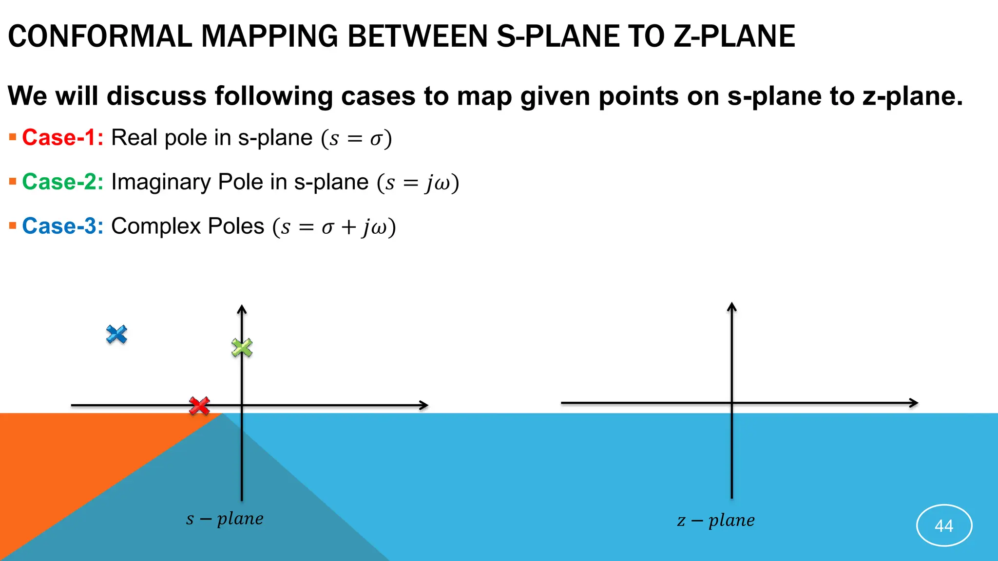
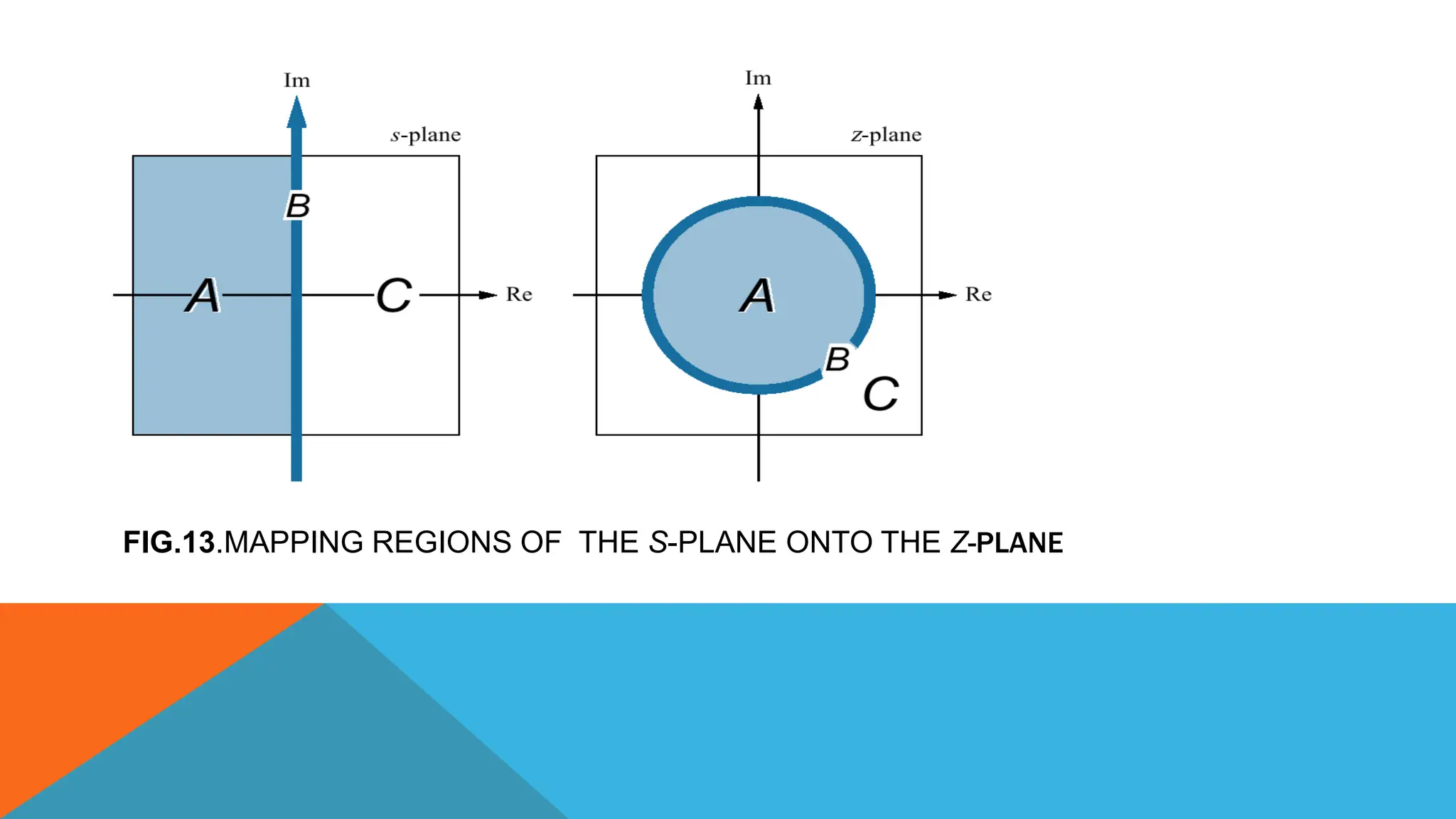
CONFORMAL MAPPING BETWEENS-PLANE TO Z-PLANE
We will discuss following cases to map given points on s-plane to z-plane.
Case-1: Real pole in s-plane (𝑠 = 𝜎)
Case-2: Imaginary Pole in s-plane (𝑠 = 𝑗𝜔)
Case-3: Complex Poles (𝑠 = 𝜎 + 𝑗𝜔)
44
𝑠 − 𝑝𝑙𝑎𝑛𝑒 𝑧 − 𝑝𝑙𝑎𝑛𝑒
45.
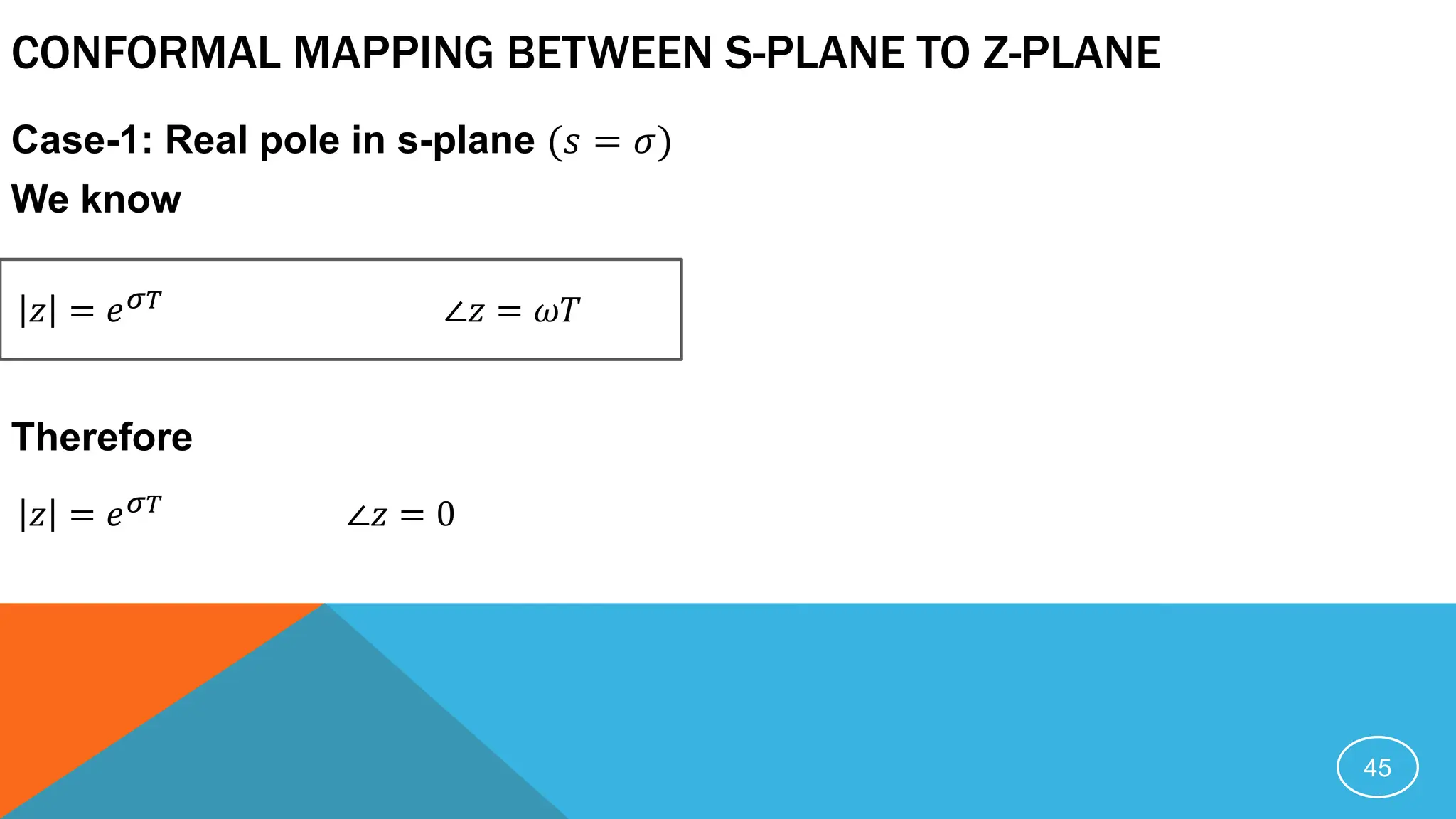
CONFORMAL MAPPING BETWEENS-PLANE TO Z-PLANE
Case-1: Real pole in s-plane (𝑠 = 𝜎)
We know
Therefore
45
∠𝑧 = 𝜔𝑇
𝑧 = 𝑒𝜎𝑇
𝑧 = 𝑒𝜎𝑇 ∠𝑧 = 0
46.
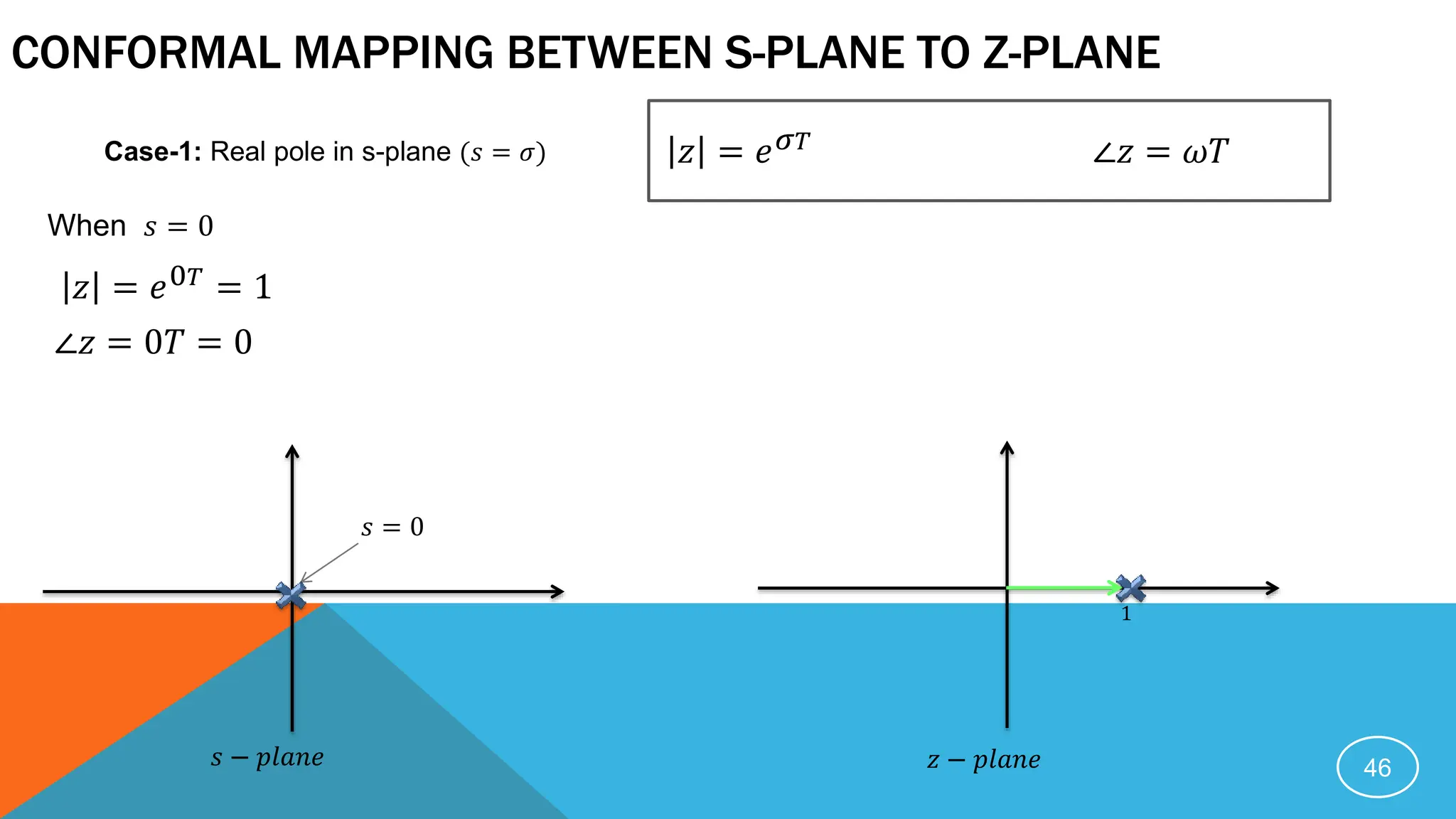
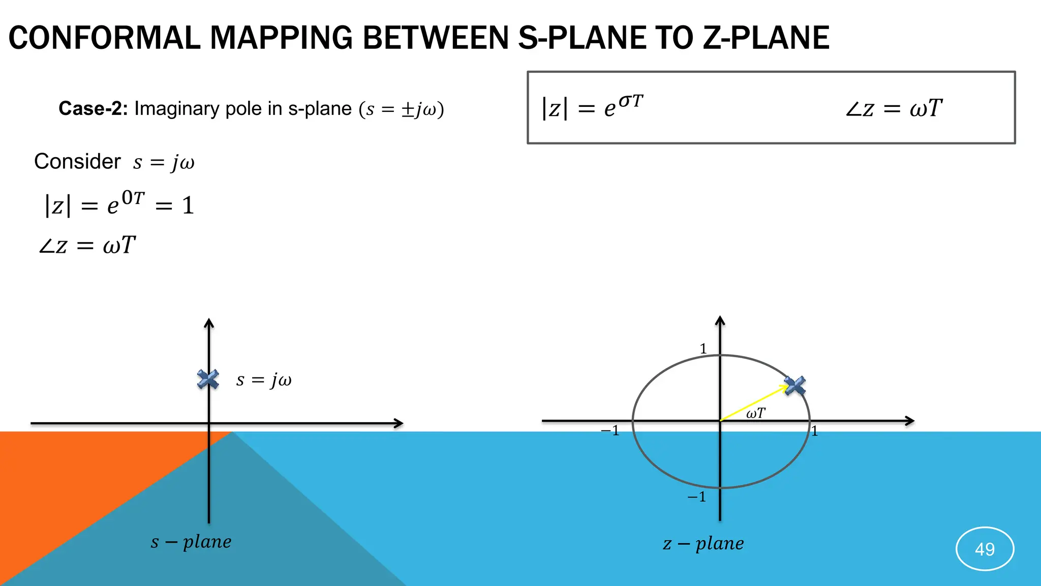
CONFORMAL MAPPING BETWEENS-PLANE TO Z-PLANE
46
When 𝑠 = 0
∠𝑧 = 𝜔𝑇
𝑧 = 𝑒𝜎𝑇
𝑧 = 𝑒0𝑇 = 1
∠𝑧 = 0𝑇 = 0
𝑠 = 0
𝑠 − 𝑝𝑙𝑎𝑛𝑒 𝑧 − 𝑝𝑙𝑎𝑛𝑒
1
Case-1: Real pole in s-plane (𝑠 = 𝜎)
47.
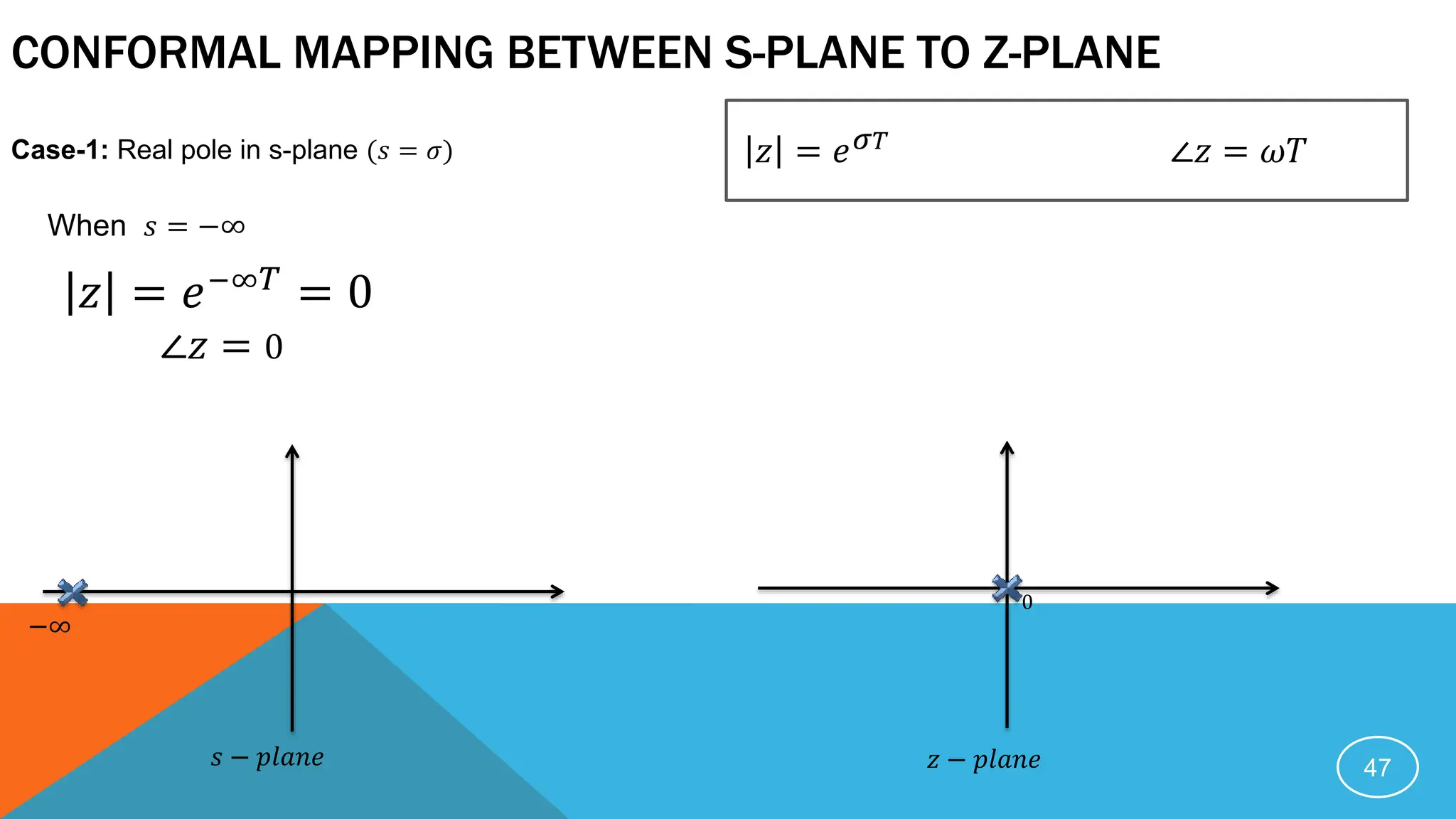
CONFORMAL MAPPING BETWEENS-PLANE TO Z-PLANE
47
When 𝑠 = −∞
∠𝑧 = 𝜔𝑇
𝑧 = 𝑒𝜎𝑇
𝑧 = 𝑒−∞𝑇
= 0
∠𝑧 = 0
−∞
𝑠 − 𝑝𝑙𝑎𝑛𝑒 𝑧 − 𝑝𝑙𝑎𝑛𝑒
0
Case-1: Real pole in s-plane (𝑠 = 𝜎)
48.
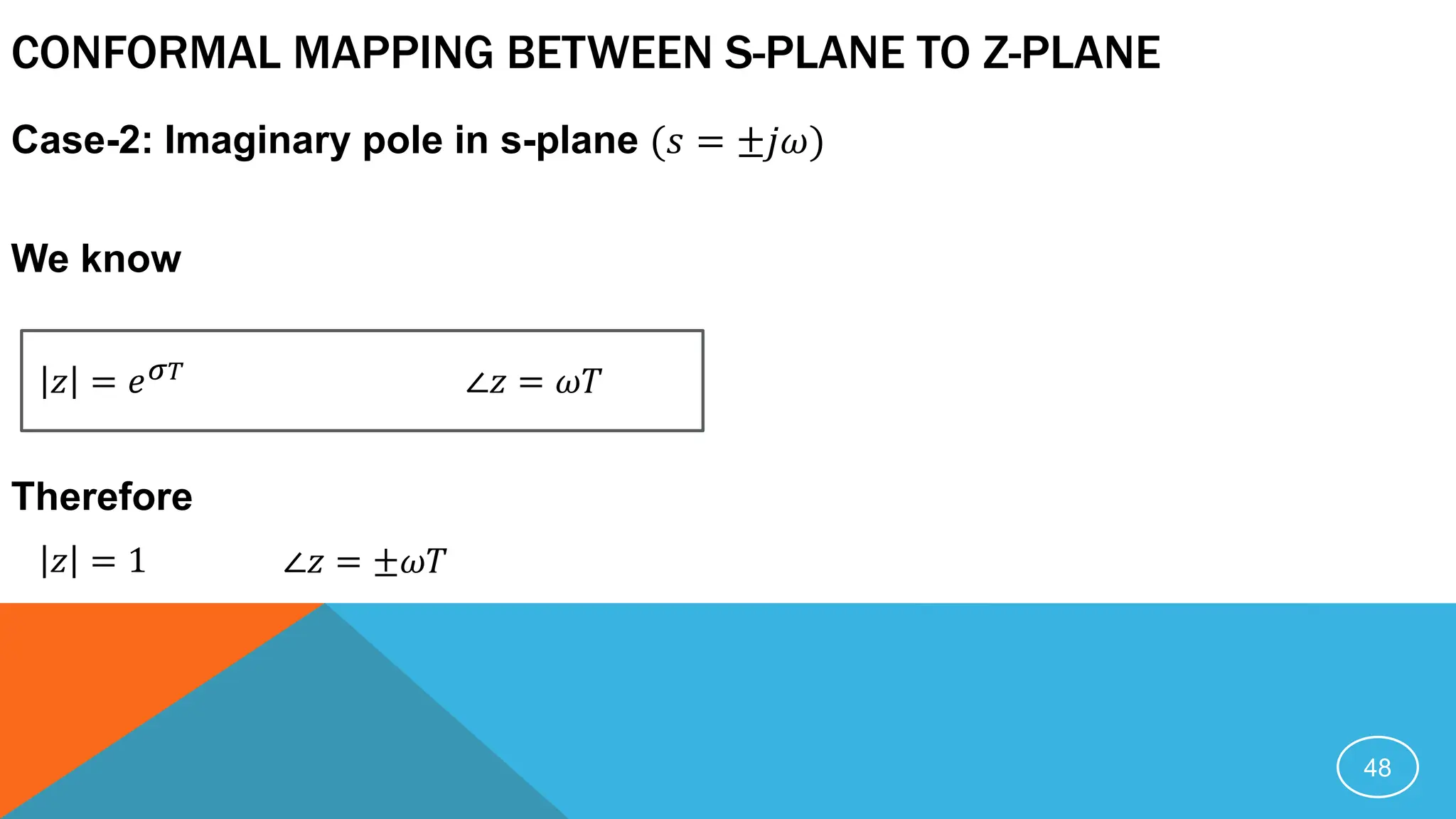
CONFORMAL MAPPING BETWEENS-PLANE TO Z-PLANE
Case-2: Imaginary pole in s-plane (𝑠 = ±𝑗𝜔)
We know
Therefore
48
∠𝑧 = 𝜔𝑇
𝑧 = 𝑒𝜎𝑇
𝑧 = 1 ∠𝑧 = ±𝜔𝑇
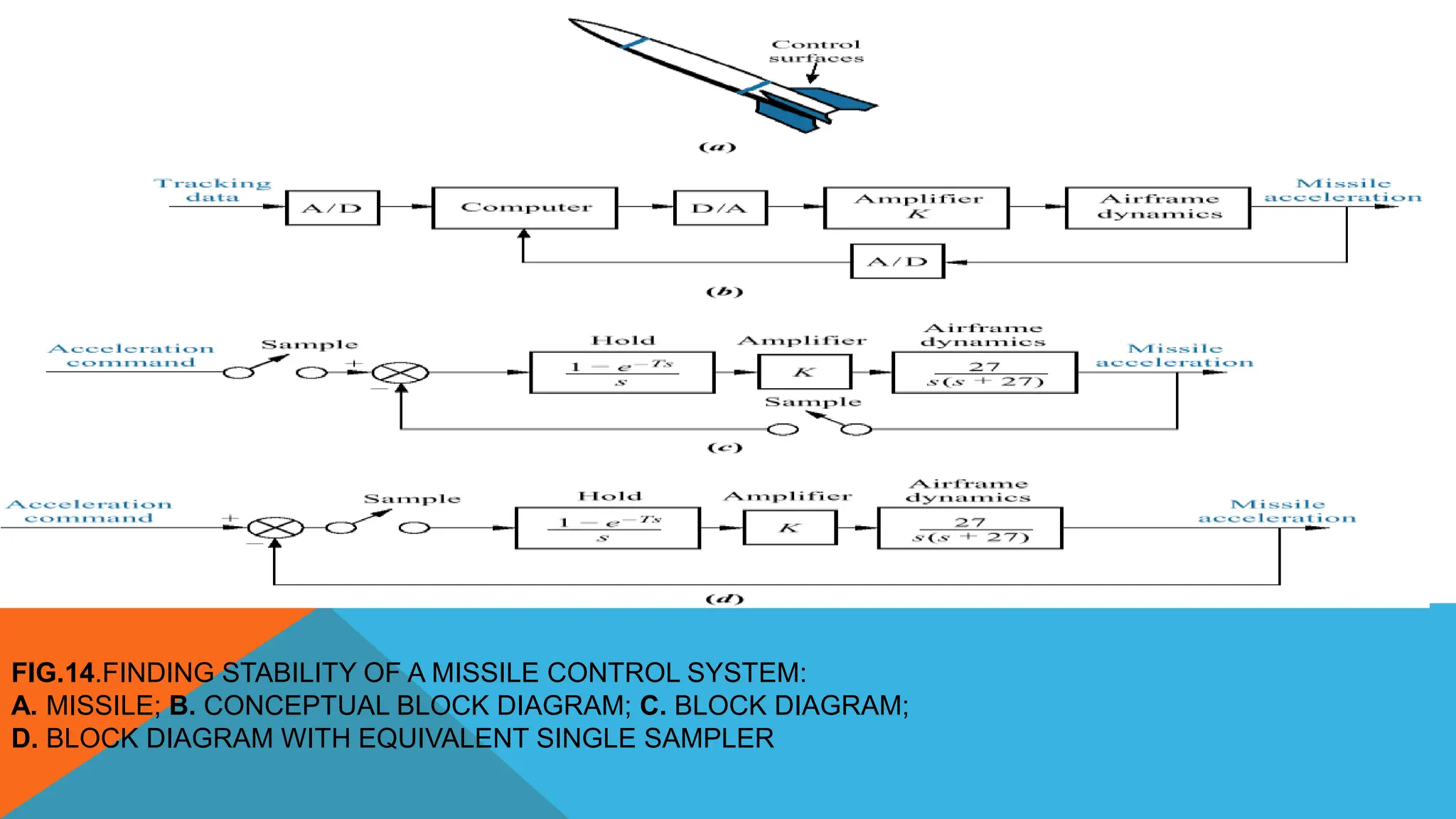
FIG.14.FINDING STABILITY OFA MISSILE CONTROL SYSTEM:
A. MISSILE; B. CONCEPTUAL BLOCK DIAGRAM; C. BLOCK DIAGRAM;
D. BLOCK DIAGRAM WITH EQUIVALENT SINGLE SAMPLER
53.
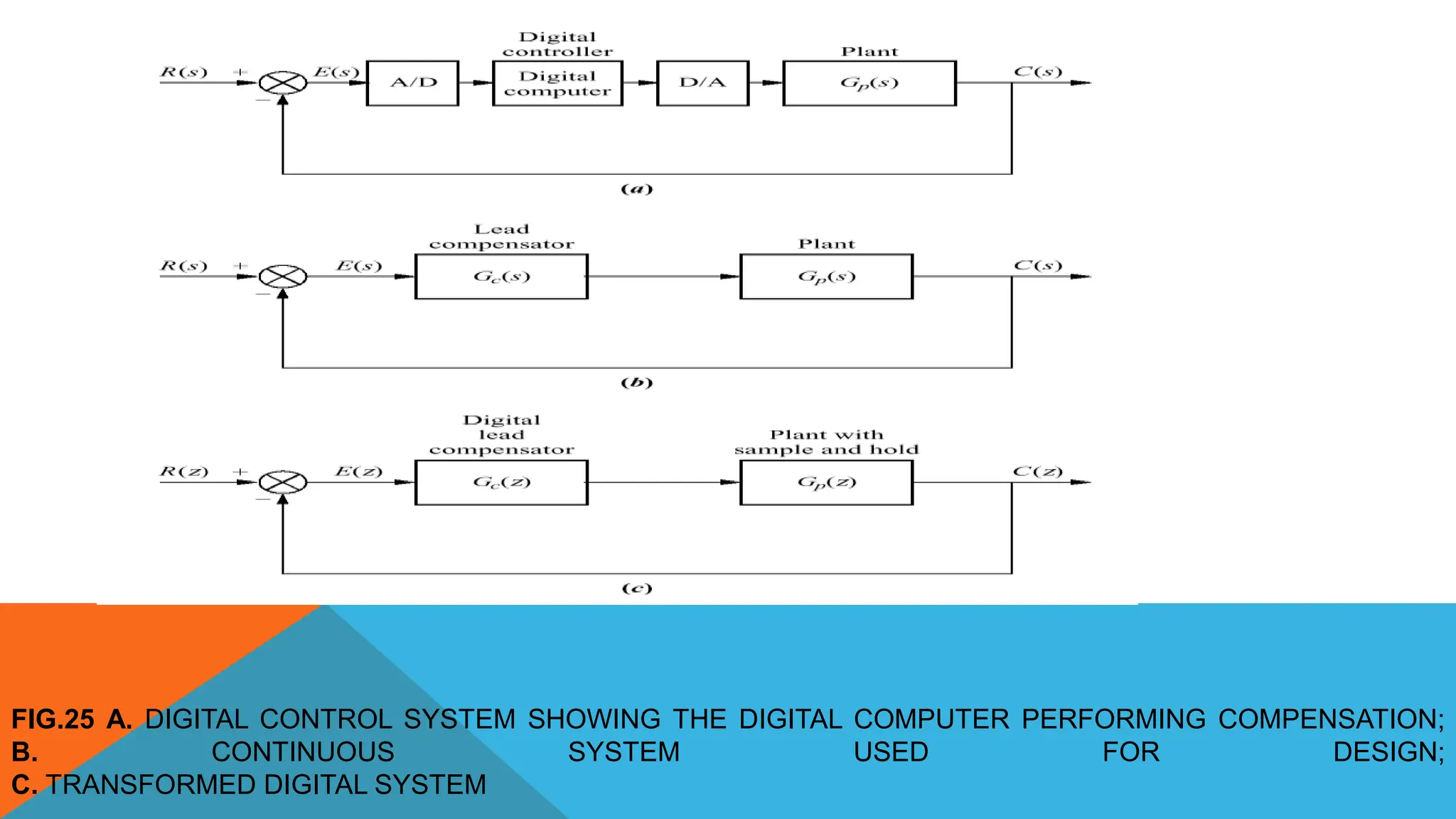
FIG.25 A. DIGITALCONTROL SYSTEM SHOWING THE DIGITAL COMPUTER PERFORMING COMPENSATION;
B. CONTINUOUS SYSTEM USED FOR DESIGN;
C. TRANSFORMED DIGITAL SYSTEM
55
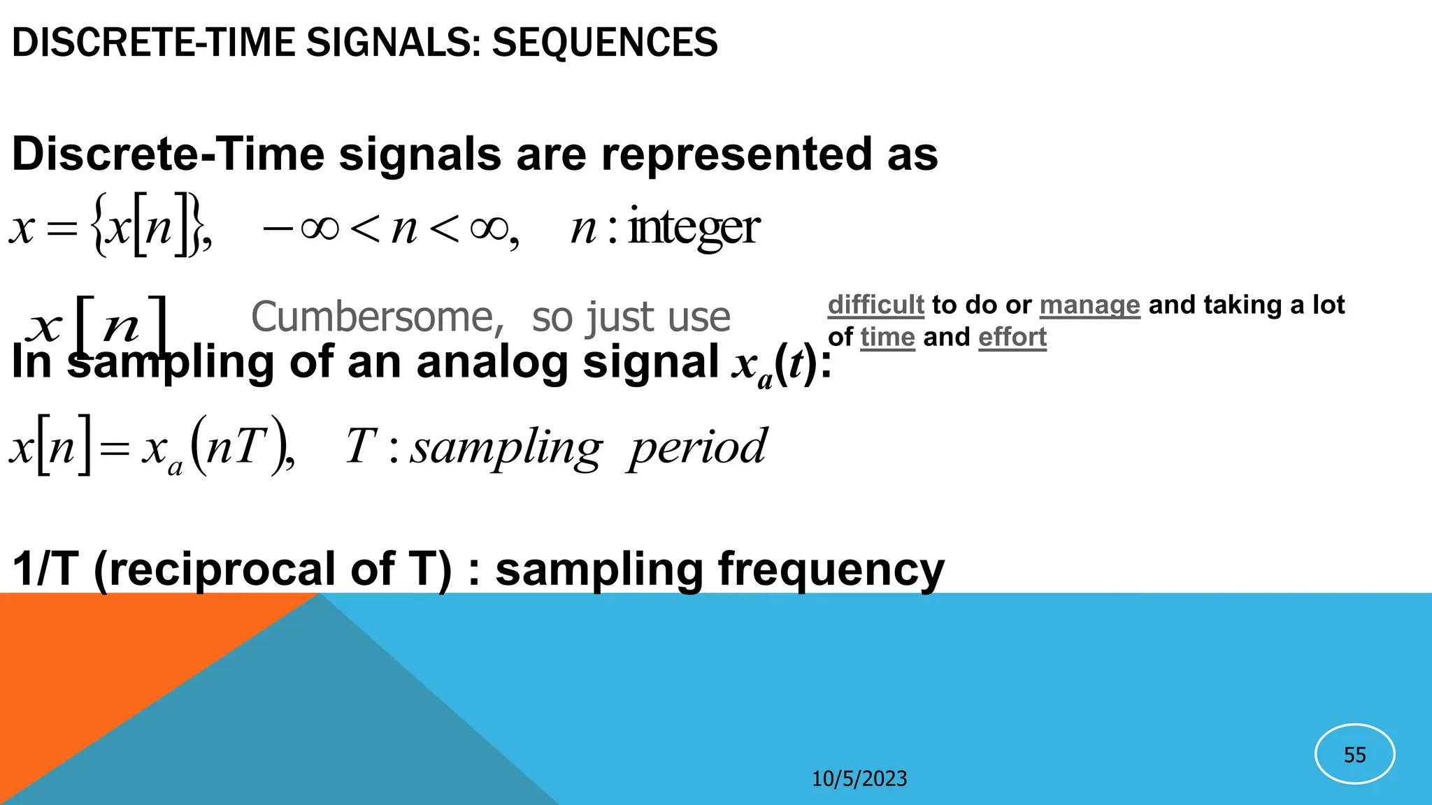
DISCRETE-TIME SIGNALS: SEQUENCES
Discrete-Timesignals are represented as
In sampling of an analog signal xa(t):
1/T (reciprocal of T) : sampling frequency
integer
:
,
, n
n
n
x
x
period
sampling
T
nT
x
n
x a :
,
10/5/2023
Cumbersome, so just use
x n
difficult to do or manage and taking a lot
of time and effort
56.
56
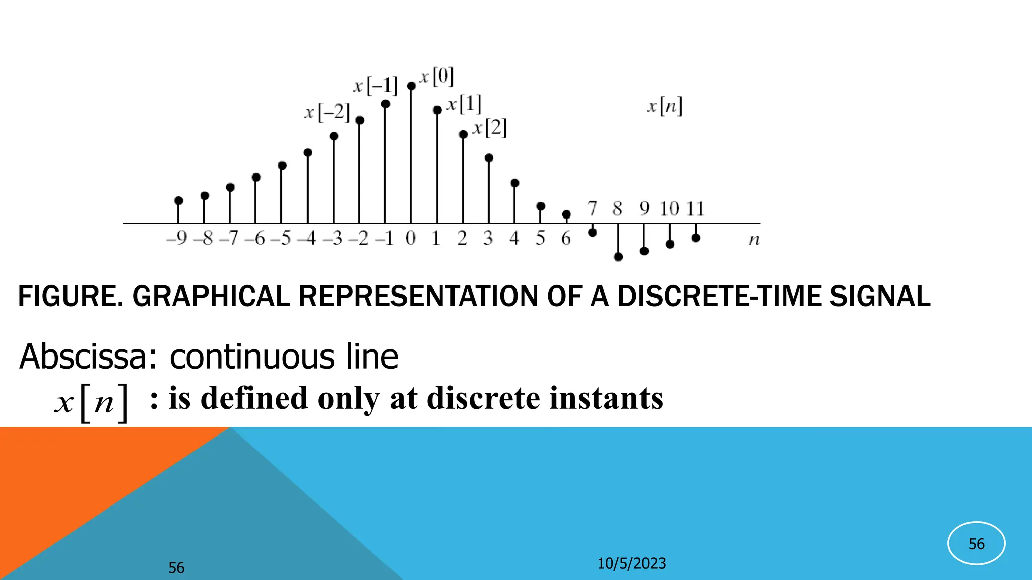
FIGURE. GRAPHICAL REPRESENTATIONOF A DISCRETE-TIME SIGNAL
10/5/2023
56
Abscissa: continuous line
: is defined only at discrete instants
x n
58 10/5/2023
58
Sum oftwo sequences
Product of two sequences
Multiplication of a sequence by a number α
Delay (shift) of a sequence
BASIC SEQUENCE OPERATIONS
]
[
]
[ n
y
n
x
integer
:
]
[
]
[ 0
0 n
n
n
x
n
y
]
[
]
[ n
y
n
x
]
[n
x
59.
59
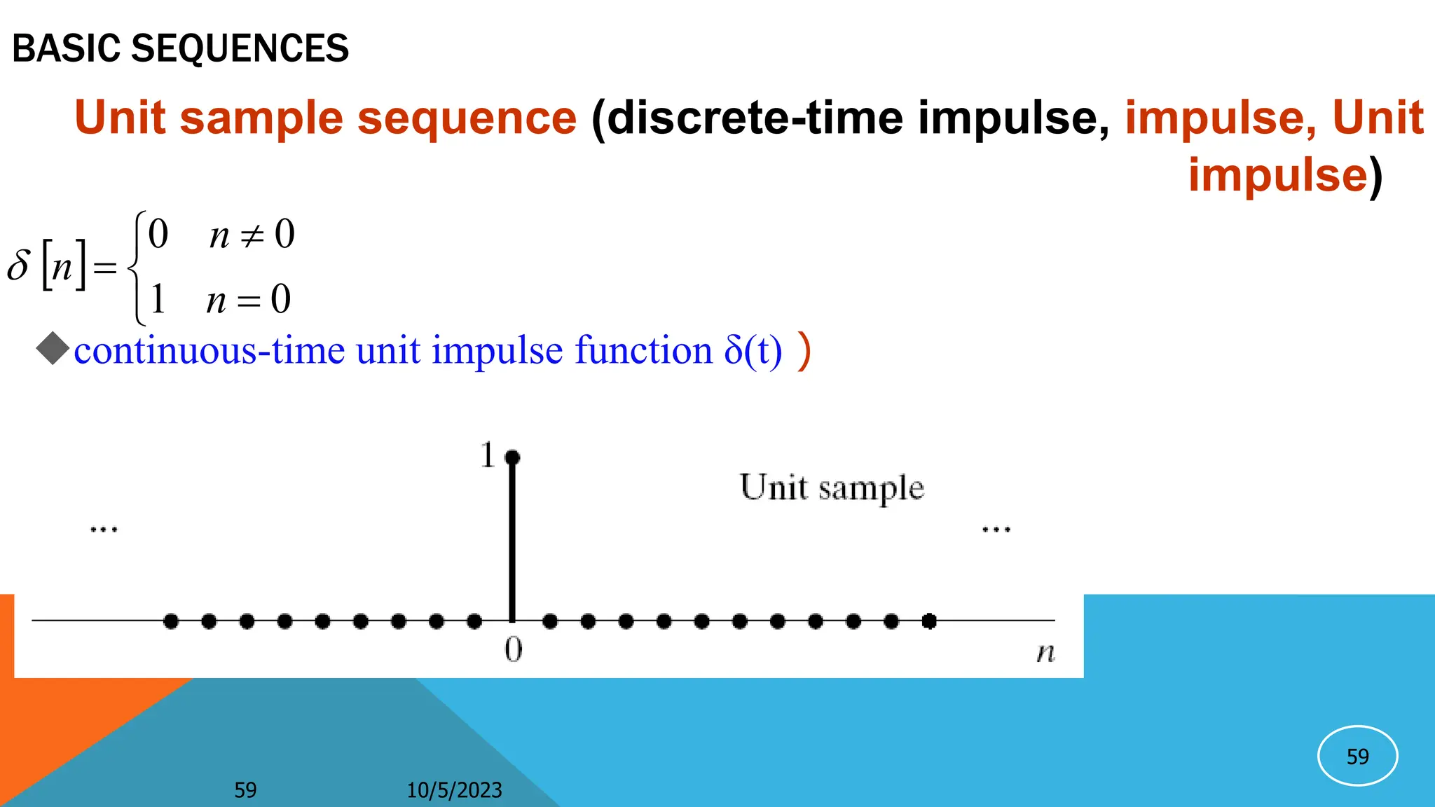
BASIC SEQUENCES
Unit samplesequence (discrete-time impulse, impulse, Unit
impulse)
0
1
0
0
n
n
n
10/5/2023
59
continuous-time unit impulse function δ(t) )
60.
60
BASIC SEQUENCES
[ ][ ] [ ]
k
x n x k n k
7
2
1
3 7
2
1
3
n
a
n
a
n
a
n
a
n
p
10/5/2023
60
arbitrary sequence
A sum of scaled, delayed impulses
61.
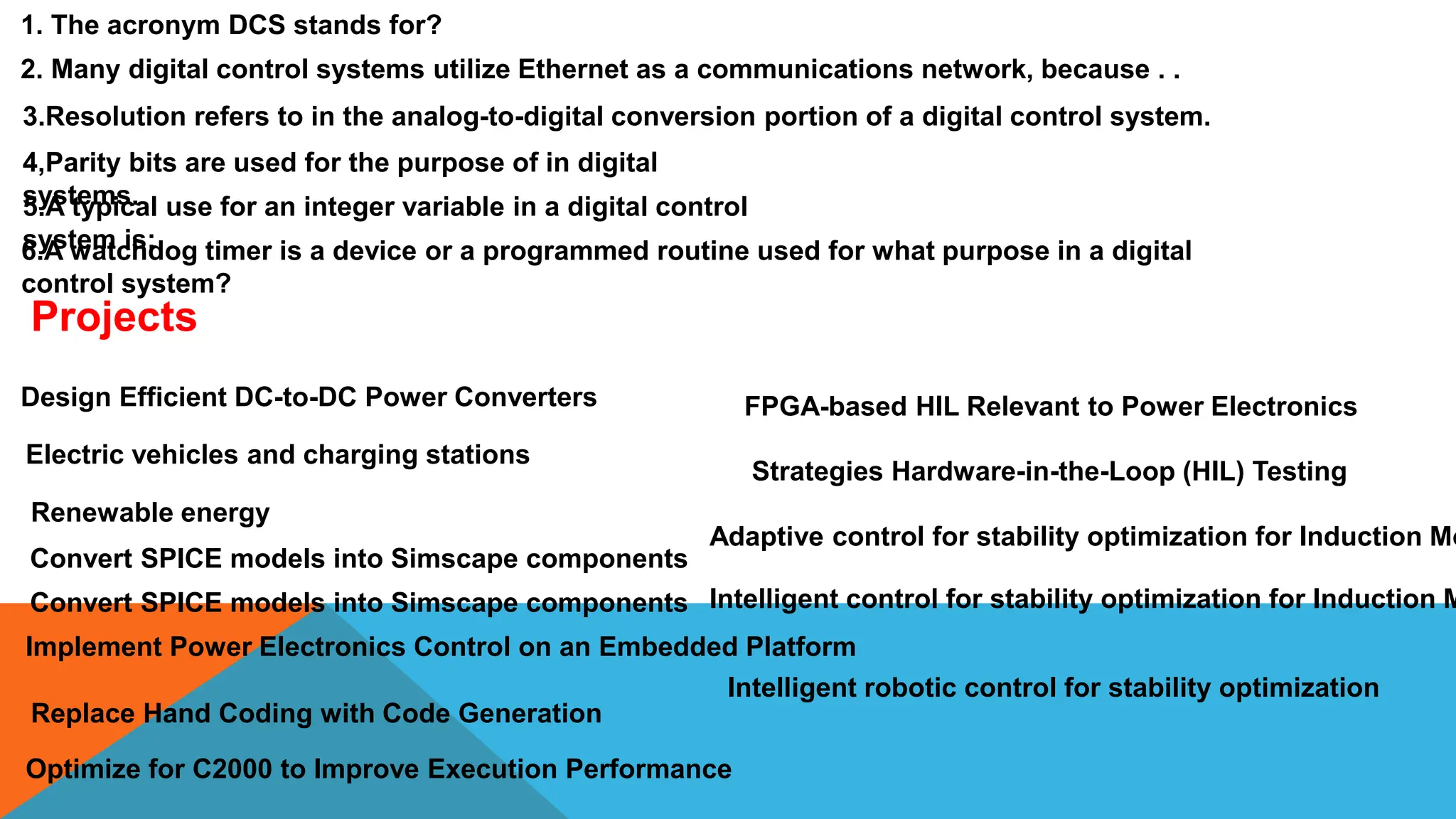
1. The acronymDCS stands for?
2. Many digital control systems utilize Ethernet as a communications network, because . .
3.Resolution refers to in the analog-to-digital conversion portion of a digital control system.
4,Parity bits are used for the purpose of in digital
systems.
5.A typical use for an integer variable in a digital control
system is:
6.A watchdog timer is a device or a programmed routine used for what purpose in a digital
control system?
Projects
Design Efficient DC-to-DC Power Converters
Electric vehicles and charging stations
Renewable energy
Convert SPICE models into Simscape components
Convert SPICE models into Simscape components
Implement Power Electronics Control on an Embedded Platform
Replace Hand Coding with Code Generation
Optimize for C2000 to Improve Execution Performance
Strategies Hardware-in-the-Loop (HIL) Testing
FPGA-based HIL Relevant to Power Electronics
Adaptive control for stability optimization for Induction Mo
Intelligent control for stability optimization for Induction M
Intelligent robotic control for stability optimization

![57
Figure 2
EXAMPLE Sampling the analog waveform
)
(
|
)
(
]
[ nT
x
t
x
n
x a
nT
t
a
](https://image.slidesharecdn.com/lecture1digitalcontrolsystems-231005170707-1293f408/75/Lecture-_1_-Digital-Control-Systems-pptx-57-2048.jpg)
![58 10/5/2023
58
Sum of two sequences
Product of two sequences
Multiplication of a sequence by a number α
Delay (shift) of a sequence
BASIC SEQUENCE OPERATIONS
]
[
]
[ n
y
n
x
integer
:
]
[
]
[ 0
0 n
n
n
x
n
y
]
[
]
[ n
y
n
x
]
[n
x
](https://image.slidesharecdn.com/lecture1digitalcontrolsystems-231005170707-1293f408/75/Lecture-_1_-Digital-Control-Systems-pptx-58-2048.jpg)
![60
BASIC SEQUENCES
[ ] [ ] [ ]
k
x n x k n k
7
2
1
3 7
2
1
3
n
a
n
a
n
a
n
a
n
p
10/5/2023
60
arbitrary sequence
A sum of scaled, delayed impulses](https://image.slidesharecdn.com/lecture1digitalcontrolsystems-231005170707-1293f408/75/Lecture-_1_-Digital-Control-Systems-pptx-60-2048.jpg)