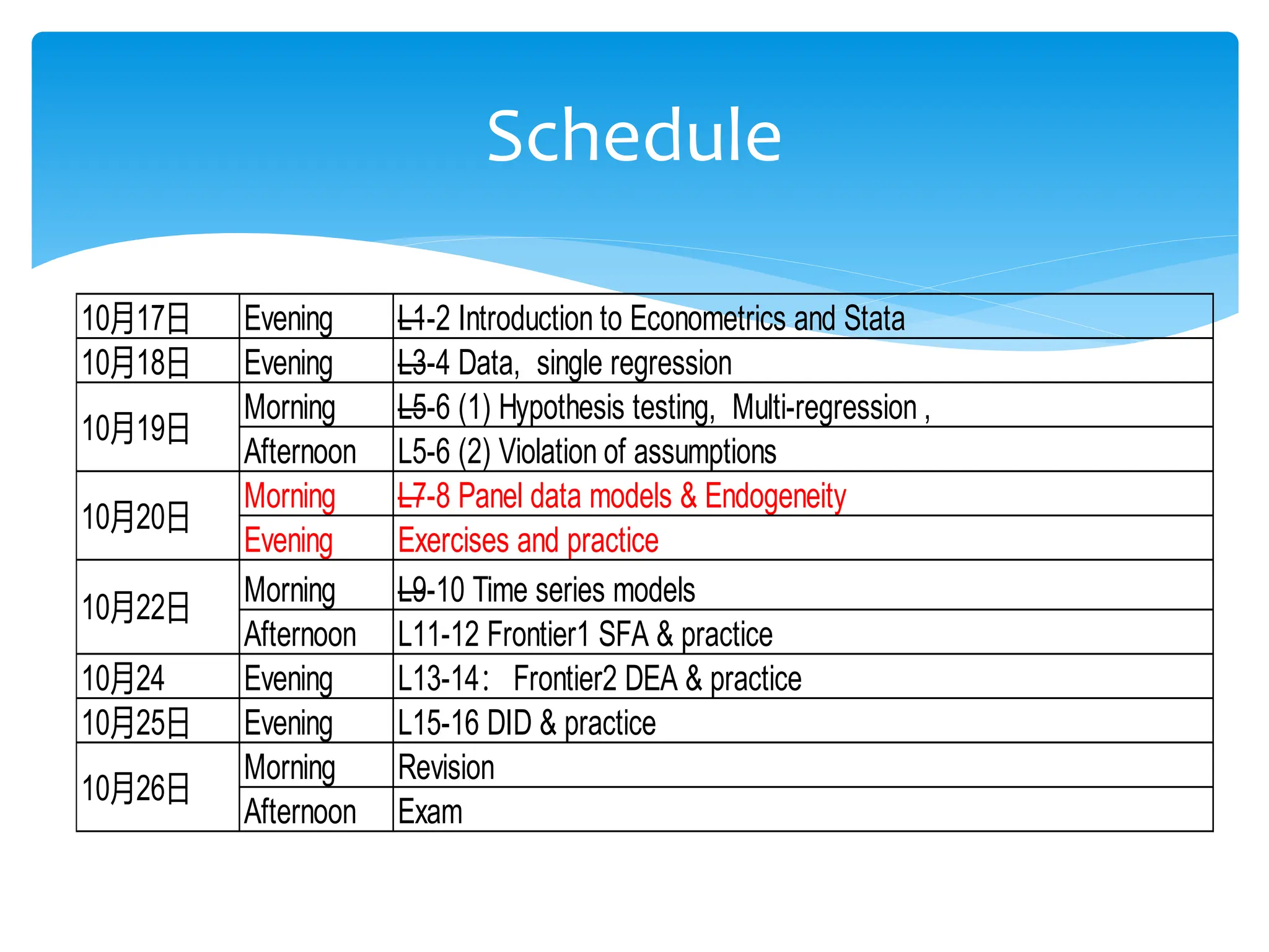
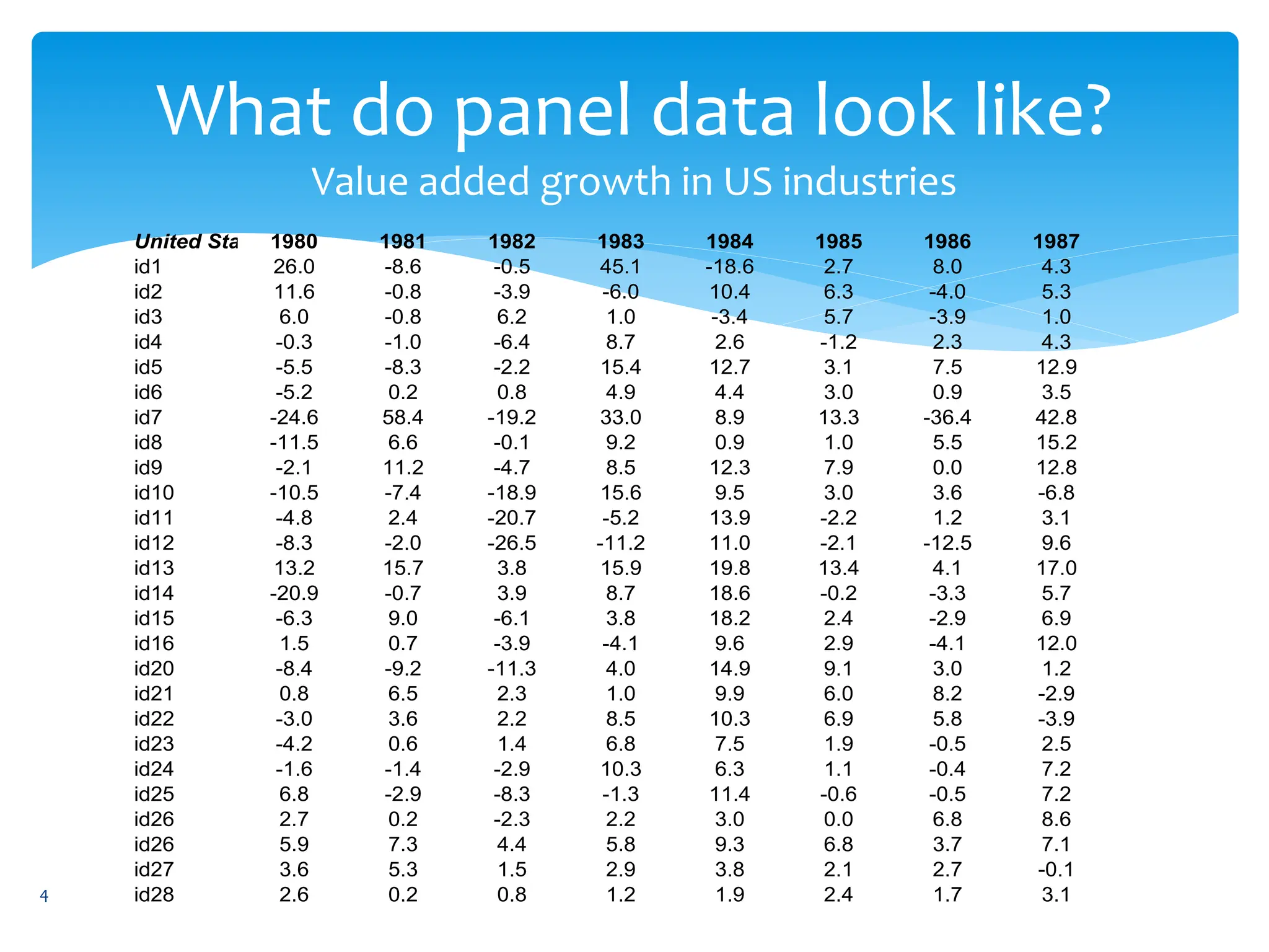
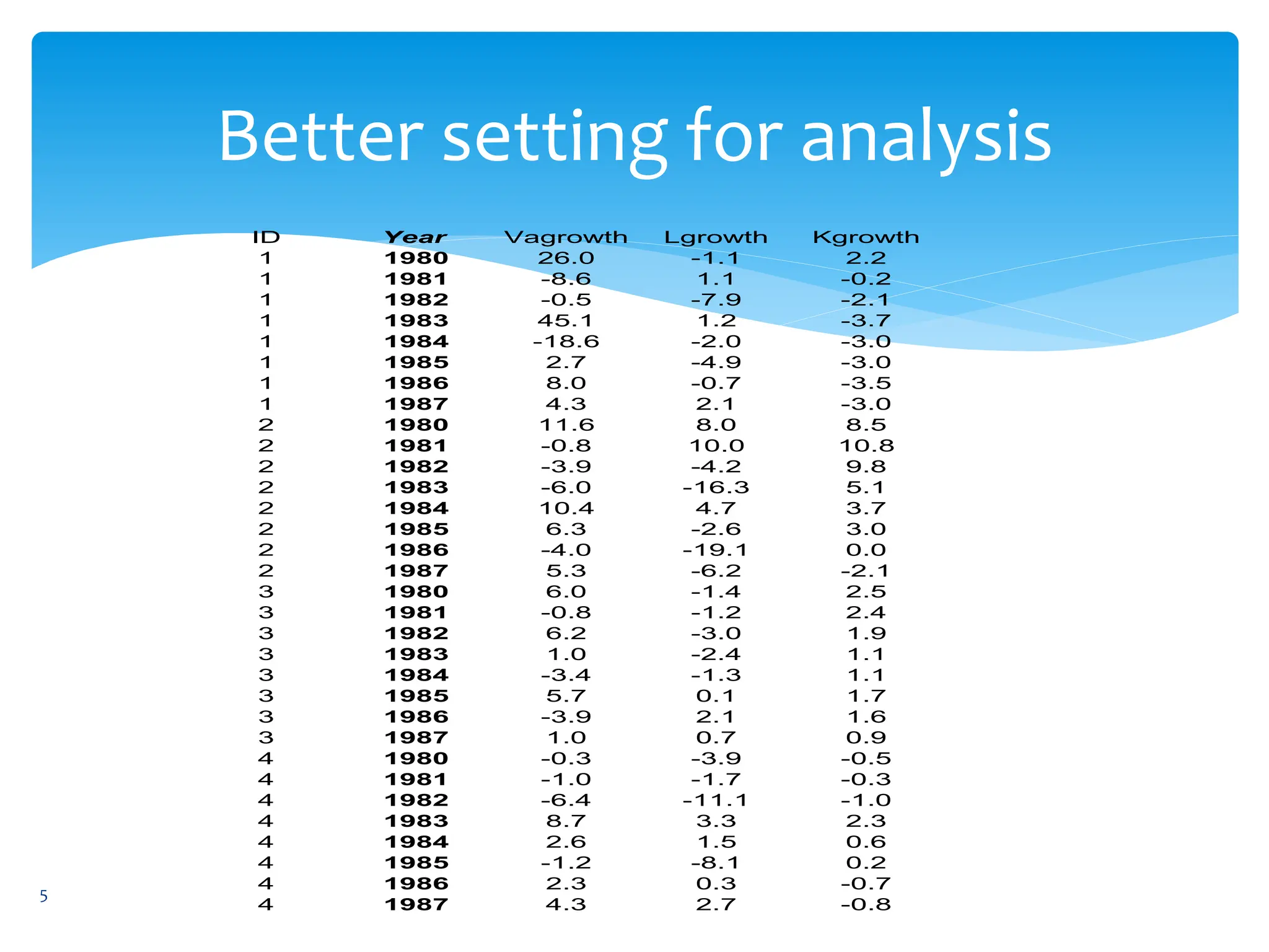
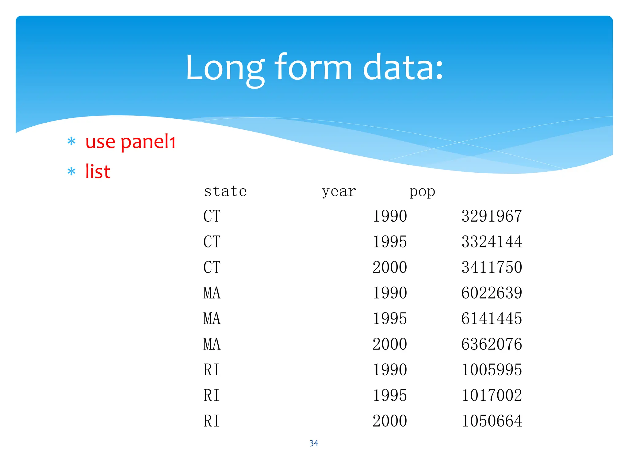
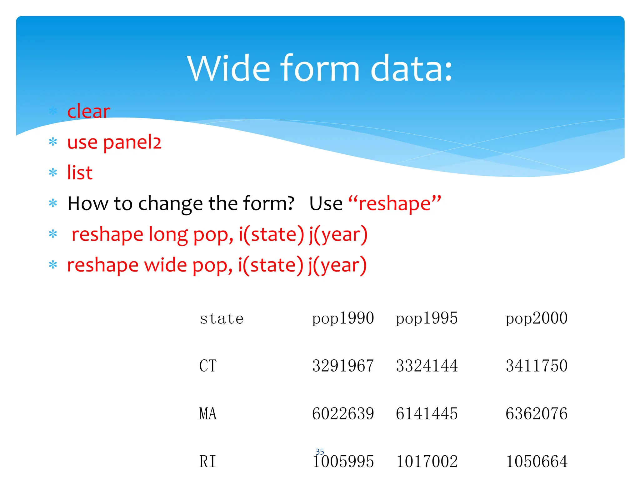
This document provides an overview of a panel data analysis course, including: - The schedule, which covers topics like panel data models, endogeneity, time series models, and difference-in-differences. - An explanation of panel data, which has multiple cross-sections observed over time, and how it can be balanced or unbalanced. - Examples of how panel data is structured and why it is useful for studying dynamic changes and effects not seen in cross-section or time series data alone. 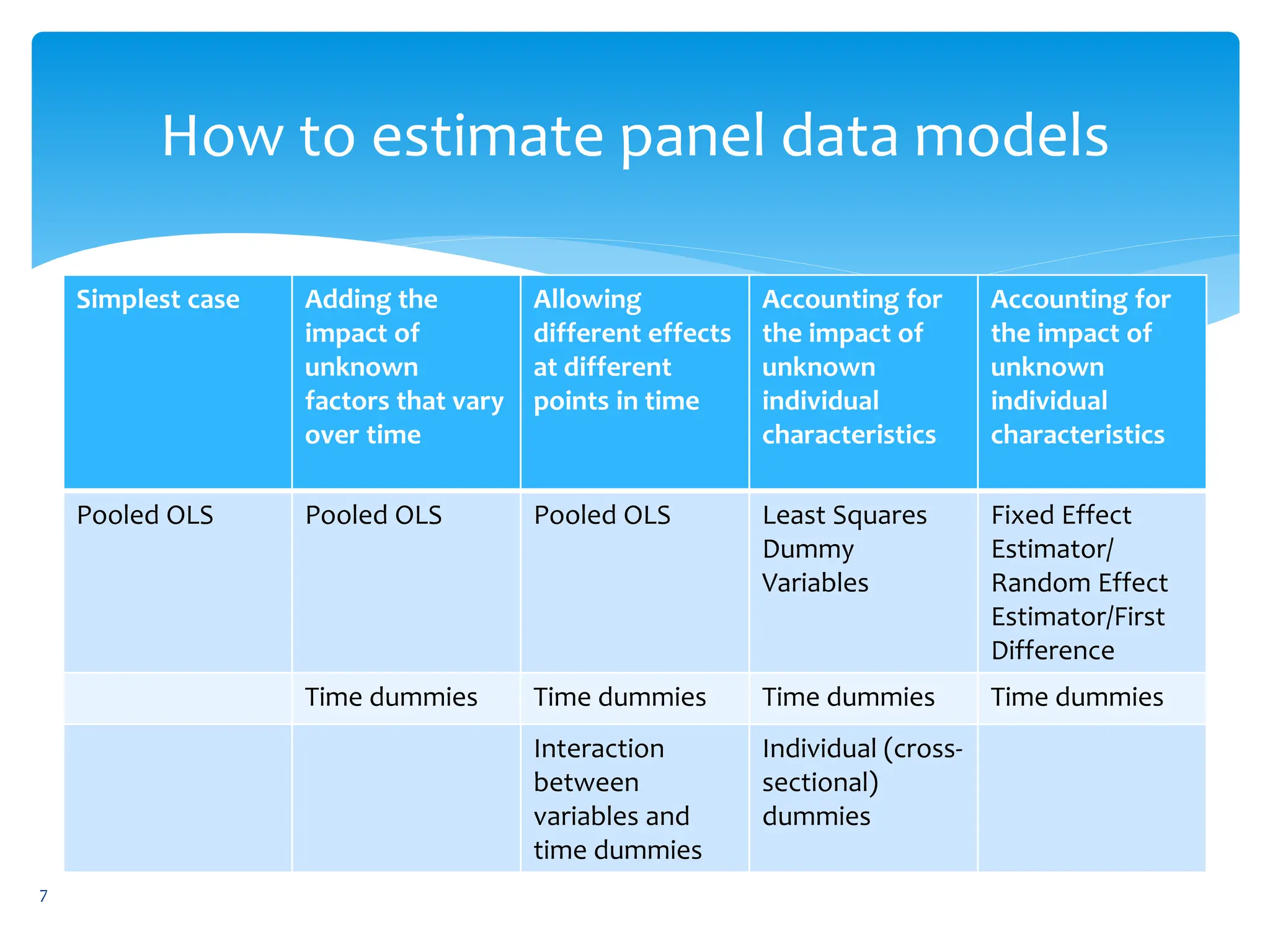- Methods for estimating panel data models, ranging from simple pooled OLS to fixed effects and random effects models.

1. Advanced econometrics and Stata
L7-8 Panel Data Analysis
Dr. Chunxia Jiang
Business School, University of Aberdeen, UK
Beijing , 17-26 Nov 2019

2. Schedule
10月17日 Evening —
L1-2 Introduction to Econometrics and Stata
10月18日 Evening —
L3-4 Data, single regression
Morning —
L5-6 (1) Hypothesis testing, Multi-regression ,
Afternoon L5-6 (2) Violation of assumptions
Morning —
L7-8 Panel data models & Endogeneity
Evening Exercises and practice
Morning —
L9-10 Time series models
Afternoon L11-12 Frontier1 SFA & practice
10月24 Evening L13-14： Frontier2 DEA & practice
10月25日 Evening L15-16 DID & practice
Morning Revision
Afternoon Exam
10月20日
10月19日
10月22日
10月26日

3. Analysis of panel data.
 A panel data set has several cross sections (industries,
companies, workers) observed over a certain period of time.
 Normally we repeat the observations for the same unit, i.e.
we follow individuals/firms/ cities over time.
 Balanced panel: we have the same time period (T) for each
cross sectional unit (N).
 Unbalanced panel: some of the time periods are missing.
 We do not have to have observations every year to obtain a
panel.
 We could observe a certain phenomenon every 5 years, for
example.
3

4. What do panel data look like?
Value added growth in US industries
United States1980 1981 1982 1983 1984 1985 1986 1987
id1 26.0 -8.6 -0.5 45.1 -18.6 2.7 8.0 4.3
id2 11.6 -0.8 -3.9 -6.0 10.4 6.3 -4.0 5.3
id3 6.0 -0.8 6.2 1.0 -3.4 5.7 -3.9 1.0
id4 -0.3 -1.0 -6.4 8.7 2.6 -1.2 2.3 4.3
id5 -5.5 -8.3 -2.2 15.4 12.7 3.1 7.5 12.9
id6 -5.2 0.2 0.8 4.9 4.4 3.0 0.9 3.5
id7 -24.6 58.4 -19.2 33.0 8.9 13.3 -36.4 42.8
id8 -11.5 6.6 -0.1 9.2 0.9 1.0 5.5 15.2
id9 -2.1 11.2 -4.7 8.5 12.3 7.9 0.0 12.8
id10 -10.5 -7.4 -18.9 15.6 9.5 3.0 3.6 -6.8
id11 -4.8 2.4 -20.7 -5.2 13.9 -2.2 1.2 3.1
id12 -8.3 -2.0 -26.5 -11.2 11.0 -2.1 -12.5 9.6
id13 13.2 15.7 3.8 15.9 19.8 13.4 4.1 17.0
id14 -20.9 -0.7 3.9 8.7 18.6 -0.2 -3.3 5.7
id15 -6.3 9.0 -6.1 3.8 18.2 2.4 -2.9 6.9
id16 1.5 0.7 -3.9 -4.1 9.6 2.9 -4.1 12.0
id20 -8.4 -9.2 -11.3 4.0 14.9 9.1 3.0 1.2
id21 0.8 6.5 2.3 1.0 9.9 6.0 8.2 -2.9
id22 -3.0 3.6 2.2 8.5 10.3 6.9 5.8 -3.9
id23 -4.2 0.6 1.4 6.8 7.5 1.9 -0.5 2.5
id24 -1.6 -1.4 -2.9 10.3 6.3 1.1 -0.4 7.2
id25 6.8 -2.9 -8.3 -1.3 11.4 -0.6 -0.5 7.2
id26 2.7 0.2 -2.3 2.2 3.0 0.0 6.8 8.6
id26 5.9 7.3 4.4 5.8 9.3 6.8 3.7 7.1
id27 3.6 5.3 1.5 2.9 3.8 2.1 2.7 -0.1
id28 2.6 0.2 0.8 1.2 1.9 2.4 1.7 3.1
4

5. Better setting for analysis
ID Year Vagrowth Lgrowth Kgrowth
1 1980 26.0 -1.1 2.2
1 1981 -8.6 1.1 -0.2
1 1982 -0.5 -7.9 -2.1
1 1983 45.1 1.2 -3.7
1 1984 -18.6 -2.0 -3.0
1 1985 2.7 -4.9 -3.0
1 1986 8.0 -0.7 -3.5
1 1987 4.3 2.1 -3.0
2 1980 11.6 8.0 8.5
2 1981 -0.8 10.0 10.8
2 1982 -3.9 -4.2 9.8
2 1983 -6.0 -16.3 5.1
2 1984 10.4 4.7 3.7
2 1985 6.3 -2.6 3.0
2 1986 -4.0 -19.1 0.0
2 1987 5.3 -6.2 -2.1
3 1980 6.0 -1.4 2.5
3 1981 -0.8 -1.2 2.4
3 1982 6.2 -3.0 1.9
3 1983 1.0 -2.4 1.1
3 1984 -3.4 -1.3 1.1
3 1985 5.7 0.1 1.7
3 1986 -3.9 2.1 1.6
3 1987 1.0 0.7 0.9
4 1980 -0.3 -3.9 -0.5
4 1981 -1.0 -1.7 -0.3
4 1982 -6.4 -11.1 -1.0
4 1983 8.7 3.3 2.3
4 1984 2.6 1.5 0.6
4 1985 -1.2 -8.1 0.2
4 1986 2.3 0.3 -0.7
4 1987 4.3 2.7 -0.8
5

6. Why panel data
 The techniques of panel data estimation can take the
heterogeneity of units into account
 More informative data, more variability, less collinearity among
variables, more degree of freedom and more efficiency
 Panel data are better suited to study the dynamics of changes
 Panel data can better detect and measures effects that simply
cannot be observed in pure cross-section or pure time series data.
 Panel data allow for the study of more complicated behavioural
models
 Minimize the bias that might result if we aggregate individuals or
firms
6

7. How to estimate panel data models
Simplest case Adding the
impact of
unknown
factors that vary
over time
Allowing
different effects
at different
points in time
Accounting for
the impact of
unknown
individual
characteristics
Accounting for
the impact of
unknown
individual
characteristics
Pooled OLS Pooled OLS Pooled OLS Least Squares
Dummy
Variables
Fixed Effect
Estimator/
Random Effect
Estimator/First
Difference
Time dummies Time dummies Time dummies Time dummies
Interaction
between
variables and
time dummies
Individual (cross-
sectional)
dummies
7

8. How do we estimate panel data?
 Simplest case: we pooled all the data together, and
apply OLS to the pooled data set.
 Normally we allow for factors that change over time
but are the same for all cross sections, by adding year
dummies to the specification
 These are a set of dummies equal 1 for a particular year and
zero for any other year.
 We include only T-1 dummies – the intercept accounts for the
first year.
 We may or may not be interested in the coefficients on the
year dummies.
8

9. Panel data model – pooled OLS
Yit = a + βXit +uit Model with no time dummies
Yit = a + βXit +∑dt+uit Model with time dummies
9

10. Panel data set with year dummies
ID Year Vagrowth Lgrowth Kgrowth D1980 D1981 D1982 D1983
1 1980 26.0 -1.1 2.2 1 0 0 0
1 1981 -8.6 1.1 -0.2 0 1 0 0
1 1982 -0.5 -7.9 -2.1 0 0 1 0
1 1983 45.1 1.2 -3.7 0 0 0 1
1 1984 -18.6 -2.0 -3.0 0 0 0 0
1 1985 2.7 -4.9 -3.0 0 0 0 0
1 1986 8.0 -0.7 -3.5 0 0 0 0
1 1987 4.3 2.1 -3.0 0 0 0 0
2 1980 11.6 8.0 8.5 1 0 0 0
2 1981 -0.8 10.0 10.8 0 1 0 0
2 1982 -3.9 -4.2 9.8 0 0 1 0
2 1983 -6.0 -16.3 5.1 0 0 0 1
2 1984 10.4 4.7 3.7 0 0 0 0
2 1985 6.3 -2.6 3.0 0 0 0 0
2 1986 -4.0 -19.1 0.0 0 0 0 0
2 1987 5.3 -6.2 -2.1 0 0 0 0
3 1980 6.0 -1.4 2.5 1 0 0 0
3 1981 -0.8 -1.2 2.4 0 1 0 0
3 1982 6.2 -3.0 1.9 0 0 1 0
3 1983 1.0 -2.4 1.1 0 0 0 1
3 1984 -3.4 -1.3 1.1 0 0 0 0
3 1985 5.7 0.1 1.7 0 0 0 0
3 1986 -3.9 2.1 1.6 0 0 0 0
3 1987 1.0 0.7 0.9 0 0 0 0
4 1980 -0.3 -3.9 -0.5 1 0 0 0
4 1981 -1.0 -1.7 -0.3 0 1 0 0
4 1982 -6.4 -11.1 -1.0 0 0 1 0
4 1983 8.7 3.3 2.3 0 0 0 1
4 1984 2.6 1.5 0.6 0 0 0 0
4 1985 -1.2 -8.1 0.2 0 0 0 0
4 1986 2.3 0.3 -0.7 0 0 0 0
4 1987 4.3 2.7 -0.8 0 0 0 0
10

11.  How to create year dummies in stata?
Question

12. Shortcomings of pooled OLS
 Constant coefficients: We assume that all
cross sections are characterised by the same
coefficients and that there are no differences
across them.
 We could allow for some heterogeneity by
using interaction dummies (similarly to a cross
section analysis).
12

13. Specification of the pooled model with
time/year dummies
 A simple example with two time series observations (1978 and 1985) and
542 cross sections. A wage equation in the panel dimension:
 Only two years, we need one time dummy for the year 1985.
 We interact the variable educ with the year dummy so that beta1 gives us
the returns to education in 1978 and delta1 + beta1 the returns to
education in 1985.
 A dummy for female workers, beta 5. This captures the difference in
wages between men and women in 1978. The differential in 1985 is given
by beta5 + delta2, the latter being the interaction between the female
dummy and the year dummy.
 In this specification we are trying to capture changes across groups of
individual (male and female workers) and changes over time.
it
it
it
it
it
u
female
y
female
union
er
er
educ
y
educ
y
wage











*
85
exp
exp
*
85
85
)
log(
2
5
4
2
3
2
1
1
0
0









13

14. The Dummy variable regression
 We want to account for differences across
individuals
 We could also add a dummy for each cross sectional unit
to account for any factor that changes across each unit
but not over time.
 For example, we could have a dummy for each individual
in our wage equation example. In this way any individual
characteristic that we cannot explicitly model is
captured by the individual dummy.
 If we were using company/industry data we could have
a dummy for each company/industry.
14

15. Least Square Dummy Variable
 Yit = ai + βXit +uit LSDV
 There is an intercept for each cross sectional unit
 Yit = ai + βXit +∑dt+uit LSDV with time dummies
15

16. Shortcomings of the dummy variable
regression
 Adding a dummy for each unit creates problem in the
estimation because we need to estimate a large
number of parameters.
 The problem is particularly serious when there are a
large number of cross sections. In this case it is not
possible to run the estimation.
 However, there is a solution to this problem that allows
to account for each individual characteristic but
without the need to introduce a large number of
dummy variables.
16

17. Fixed Effect model
 This implies a simple transformation of the data (usually done
directly by your software).
 Let’s start from the following model for a single cross section,
i:
 Then let’s take the average of this equation over time:


 Now let’s subtract (2) from (1):
it
it
i
it u
x
a
y 

 1
 (1)
i
i
i
i u
x
a
y 

 1
 (2)
i
it
i
it
i
it u
u
x
x
y
y 



 )
(
1
 (3)
17

18. Fixed effect model
 Equation (3) is the transformed model. This is also called the
model with time demeaned data or within transformation.
 Very important: we no longer have the individual effects ai.
These have been dropped due to the transformation we
have applied to the data.
 We can now use OLS to estimate our transformed equation.
 Warning: we cannot include variables that vary only in the
cross section dimension because these will be dropped in
the transformation (ex. Female dummy).
i
it
i
it
i
it u
u
x
x
y
y 



 )
(
1
 (3)
18

19. Pooled
OLS
Dummy
variable
regression
Fixed effect
Constant 7.070 23.84 23.370
Tot hours 0.291 0.437 0.437
Totk 0.390 0.285 0.285
Id2 -0.627
Id3 -0.168
Id4 -0.999
Id5 -1.416
Id6 0.188
Dependent variable: log of value added for the US
Industry level data
19

20.  How to run these regression in Stata?
question

21. Assumptions of the FE model
(very important!)
 The explanatory variables are independent of
the error term in all time periods.
 The FE estimator allows for the correlation
between the explanatory variables and the
individual (unobserved) effect.
 The errors are homoskedastic and serially
uncorrelated.
21

22. The first difference estimator
 An alternative way to eliminate the unobserved
individual effect is to take first differences of the data:
 Taking the variable at time t and subtract the value of the
same variable at time t-1
 For example, let’s assume that we have a panel
composed working students in our course. Let’s look at
the equation for 1 student in year 1 and year 2:
22

23. The first difference estimator
(1)
(2)
Now let’s subtract (2) from (1):
)
(
)
( 1
2
1
12
1
1
2 i
i
i
i
i
i
i u
u
x
x
a
a
y
y 





 
This can be written as:
it
it
it u
x
y 



 1

The transformation has eliminated the individual effect.
1
1
1
1
2
2
1
2
i
i
i
i
i
i
i
i
u
x
a
y
u
x
a
y








23

24. Lagged and first differenced
variables
obs inv inv_1 d_inv
1:01 33.10
1:02 45.00 33.10 11.90
1:03 77.20 45.00 32.20
1:04 44.60 77.20 -32.60
1:05 48.10 44.60 3.50
1:06 74.40 48.10 26.30
2:01 12.93
2:02 25.90 12.93 12.97
2:03 35.05 25.90 9.15
2:04 22.89 35.05 -12.16
2:05 18.84 22.89 -4.05
2:06 28.57 18.84 9.73
24

25. Characteristic of the first difference
estimator.
 We can use OLS in the model in first differences, assuming
the hypothesis underlying the OLS estimator are valid.
 Similarly to the fixed effect estimator, we are assuming
that the unobserved effect is correlated with the
explanatory variables.
 If the explanatory variables do not change over time, its
first difference equals zero. We cannot use the FD
estimator.
 The use of the FD estimator causes serious problems (bias)
if there are measurement errors in the explanatory
variables. Such errors are exacerbated when taking first
differences.
25

26. Fixed effect or first difference?
 Not easy to decide.
 T = 2, FD=FE. It does not matter which one you use.
 T>2 the estimators do not produce the same results.
Difficult to decide. One criteria is to look at the
properties of the errors:
 if uit serially uncorrelated: the FE is more efficient than FD.
 If uit is serially correlated, than FD is better (serial correlation
problem can be eliminated by taking first differences).
26

27. First difference or fixed effect?
 Another criteria is to look at the shape of the panel.
 If N is large and T is small then the FE might be a more
suitable estimator. The time series property of the data is
less important.
 If N is small and T is large looking at the time series
properties of the data is more important.
 In practice: report both results and try to explain why they
differ.
27

28. Random effect estimator
 The random effect (RE) model can be written as
follows:
 However, differently from previous models, the
error term has two components:
 The error term includes an individual effect. This
effect is random and it is assumed to be
uncorrelated with the explanatory variables (main
difference between FE and RE).
it
it
o
it v
x
y 

 1


it
i
it u
a
v 

28

29. Estimation of the RE model
 Because of the presence of the composite error term, the
problem of serial correlation always arises in RE estimation
and it can be quite serious.
 In fact, the individual effect, which is now part of the error
term, is always correlated with itself at different points in
time and this correlation does not decline over time.
 We have to use feasible GLS (Generalised Least Squares).
 This implies transforming the model so that we get rid of
the serial correlation problem.
29

30. When to use the RE model
 Shape of the panel: better to use the RE model when we
have large N and small T.
 The properties of the RE estimator with small N and large T
are still unknown.
 In practice it has been used with both types of data.
30

31. RE versus FE
 The RE model can include dummy variables (advantage
compared to the FE).
 RE: the assumption of no correlation between the
individual effect and the explanatory variables is very
strong.
 To use the RE we have to provide an explanation of
why the individual effect is uncorrelated with the
explanatory variables as this is normally an exception.
 Usually we use both estimators and we carry out a test
to show which is the more suitable to use.
 This is called the Hausman test.
31

32. Hausman test
 The null hypothesis:
 H0: the both the FE and the RE is consistent and
efficient
 H1: the RE is inconsistent
 The test has a χ2 distribution
 We reject the null if the p-value < 0.05
 Summarising: rejection of the null implies rejection
of the RE effect. In this case, use the FE.
32

33.  To define the problems of panel data management,
consider a dataset in which each variable contains
information on N panel units, each with T time-series
observations. The second dimension of panel data
need not be calendar time, but many estimation
techniques assume that it can be treated as such, so
that operations such as first differencing make sense.
 These data may be commonly stored in either the
long form or the wide form, in Stata. In the long form,
each observation has both an i and t subscript
33
Forms of panel data

34.  use panel1
 list
34
Long form data:
state year pop
CT 1990 3291967
CT 1995 3324144
CT 2000 3411750
MA 1990 6022639
MA 1995 6141445
MA 2000 6362076
RI 1990 1005995
RI 1995 1017002
RI 2000 1050664

35.  clear
 use panel2
 list
 How to change the form? Use “reshape”
 reshape long pop, i(state) j(year)
 reshape wide pop, i(state) j(year)
35
Wide form data:
state pop1990 pop1995 pop2000
CT 3291967 3324144 3411750
MA 6022639 6141445 6362076
RI 1005995 1017002 1050664

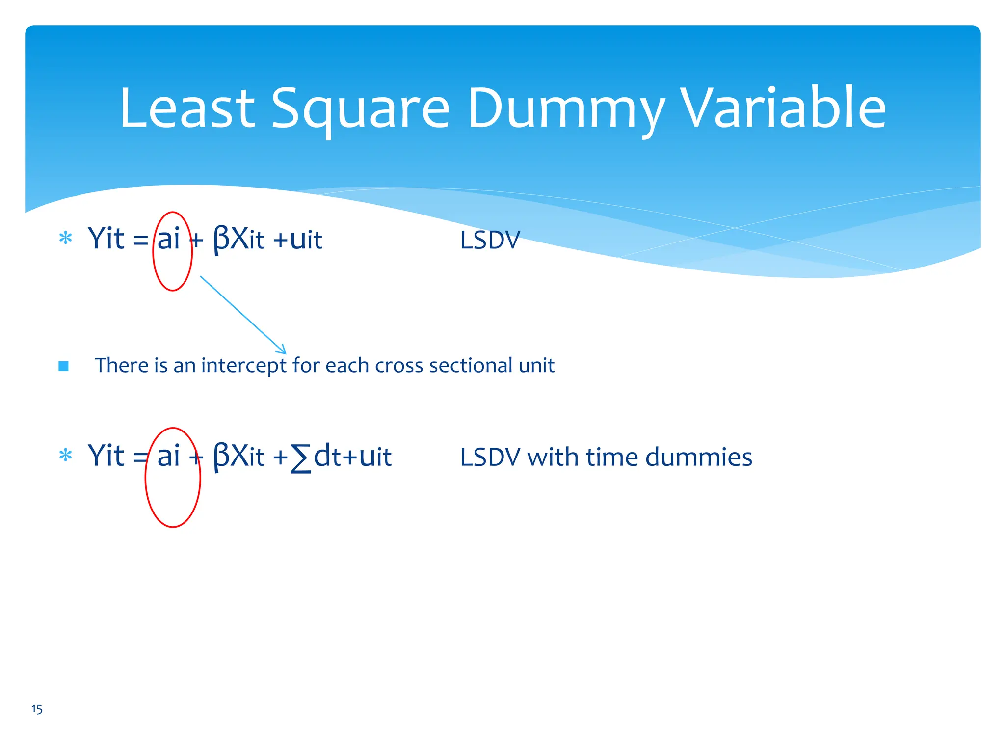
36.  restrict the slope coefficients to be constant over
both units and time, and allow for an intercept
coefficient that varies by unit or by time. For a given
observation, an intercept varying over units
 There are two interpretations of ai in this context: as a
parameter to be estimated in the model (a so-called
fixed effect) or alternatively, as a component of the
disturbance process, giving rise to a composite error
term [ai + vit ]: a so-called random effect. Under either
interpretation, ai is taken as a random variable.
36
Fixed effect estimator

37.  A one-way fixed effects model permits each cross-
sectional unit to have its own constant term while the
slope estimates (beta) are constrained across units
 This estimator is often termed the LSDV (least-
squares dummy variable) model, since it is equivalent
to including (N -1) dummy variables in the OLS
regression of y on X (including a units vector).
37
Fixed effect estimator

38.  This has the clear implication that any characteristic
which does not vary over time for each unit cannot be
included in the model: for instance, an individual’s
gender, or a firm’s three-digit SIC (industry) code. The
unit-specific intercept term absorbs all heterogeneity
in y and X that is a function of the identity of the unit,
and any variable constant over time for each unit will
be perfectly collinear with the unit’s indicator variable.
38
Fixed effect estimator

39.  xtreg depvar indepvars, fe [options]
 Use traffice data
 In this example, we have 1982–1988 state-level data for 48
U.S. states on traffic fatality rates (deaths per 100,000).
We model the highway fatality rates as a function of
several common factors: beertax, the tax on a case of beer,
spircons, a measure of spirits consumption and two
economic factors: the state unemployment rate (unrate)
andstate per capita personal income, $000 (perincK). We
present descriptive statistics for these variables of the
traffic.dta dataset.
39
Fixed effect estimator

40.  use traffic, clear
 summarize fatal beertax spircons unrate perincK
 xtreg fatal beertax spircons unrate perincK, fe
40
FE estimator example

41.  All explanatory factors are highly significant, with the
unemployment rate having a negative effect on the fatality
rate (perhaps since those who are unemployed are
income-constrained and drive fewer miles), and income a
positive effect (as expected because driving is a normal
good).
 Note the empirical correlation labeled corr(u_i, Xb) of -
0:8804. This correlation indicates that the unobserved
heterogeneity term, proxied by the estimated fixed effect,
is strongly correlated with a linear combination of the
included regressors. That is not a problem for the fixed
effects model, but as we shall see it is an important
magnitude.
41
FE estimator example

42.  We have considered one-way fixed effects models,
where the effect is attached to the individual. We may
also define a two-way fixed effect model, where
effects are attached to each unit and time period.
Stata lacks a command to estimate two-way fixed
effects models. If the number of time periods is
reasonably small, you may estimate a two-way FE
model by creating a set of time indicator variables and
including all but one in the regression.
 xtreg fatal beertax spircons unrate perincK i.year, fe
42
FE estimator example

43.  The joint test that all of the coefficients on those indicator
variables are zero will be a test of the significance of time
fixed effects. Just as the individual fixed effects (LSDV)
model requires regressors’ variation over time within each
unit, a time fixed effect (implemented with a time indicator
variable) requires regressors’ variation over units within
each time period.
 If we are estimating an equation from individual or firm
microdata, this implies that we cannot include a “macro
factor” such as the rate of GDP growth or price inflation in
a model with time fixed effects, since those factors do not
vary across individuals.
43
FE estimator example

44.  testparm i.year
 The four quantitative factors included in the one-way
fixed effects model retain their sign and significance
in the two-way fixed effects model. The time effects
are jointly significant, suggesting that they should be
included in a properly specified model. Otherwise, the
model is qualitatively similar to the earlier model, with
a sizable amount of variation explained by the
individual (state) fixed effect.
44
FE estimator example

45.  xtreg fatal beertax spircons unrate perincK, re
 In comparison to the fixed effects model, where all four
regressors were significant, we see that the beertax and
perincK variables do not have significant effects on the
fatality rate. The latter variable’s coefficient switched sign.
 The corr(u_i, Xb) in this context is assumed to be zero: a
necessary condition for the random effects estimator to
yield consistent estimates. Recall that when the fixed
effect estimator was used, this correlation was reported as
-0:8804.
45
RE estimator example

46.  A Hausman test may be used to test the null
hypothesis that the extra conditions imposed by the
random effects estimator are valid. The fixed effects
estimator, which does not impose those conditions, is
consistent regardless of the independence of the
individual effects.
46
Hausman test

47.  We may consider two alternatives in the Hausman
test framework, estimating both models and
comparing their common coefficient estimates in a
probabilistic sense. If both fixed and random effects
models generate consistent point estimates of the
slope parameters, they will not differ meaningfully.
 If the assumption of independence is violated, the
inconsistent random effects estimates will differ from
their fixed effects counterparts.
47
Hausman test

48.  To implement the Hausman test, you estimate each form
of the model, using the commands estimates store set
after each estimation, with set defining that set of
estimates: for instance, set might be fix for the fixed
effects model.
 This test is based on the difference of the two estimated
covariance matrices (which is not guaranteed to be
positive definite) and the difference between the fixed
effects and random effects vectors of slope coefficients.
48
Hausman test

49.  qui xtreg fatal beertax spircons unrate perincK, fe
 estimates store fix
 qui xtreg fatal beertax spircons unrate perincK, re
 hausman fix .
49
Hauseman test

50.  As we might expect from the quite different point
estimates generated by the random effects estimator, the
Hausman test’s null—that the random effects estimator is
consistent—is soundly rejected.
 The sizable estimated correlation reported in the fixed
effects estimator also supports this rejection. The state-
level individual effects cannot be considered independent
of the regressors: hardly surprising, given the wide
variation in some of the regressors over states.
 This illustrates the difficulty with the random effects
estimator: one rarely finds a context where it may be
employed, as the necessary assumptions are very likely to
be violated in many empirical settings.
50
Hausman

51.  Try to write command code using a do file for
estimating models we discussed today
 Practice with a dataset of your interests
 We will practice it during the seminar session
tomorrow using a dataset of mine
Seminar discussions