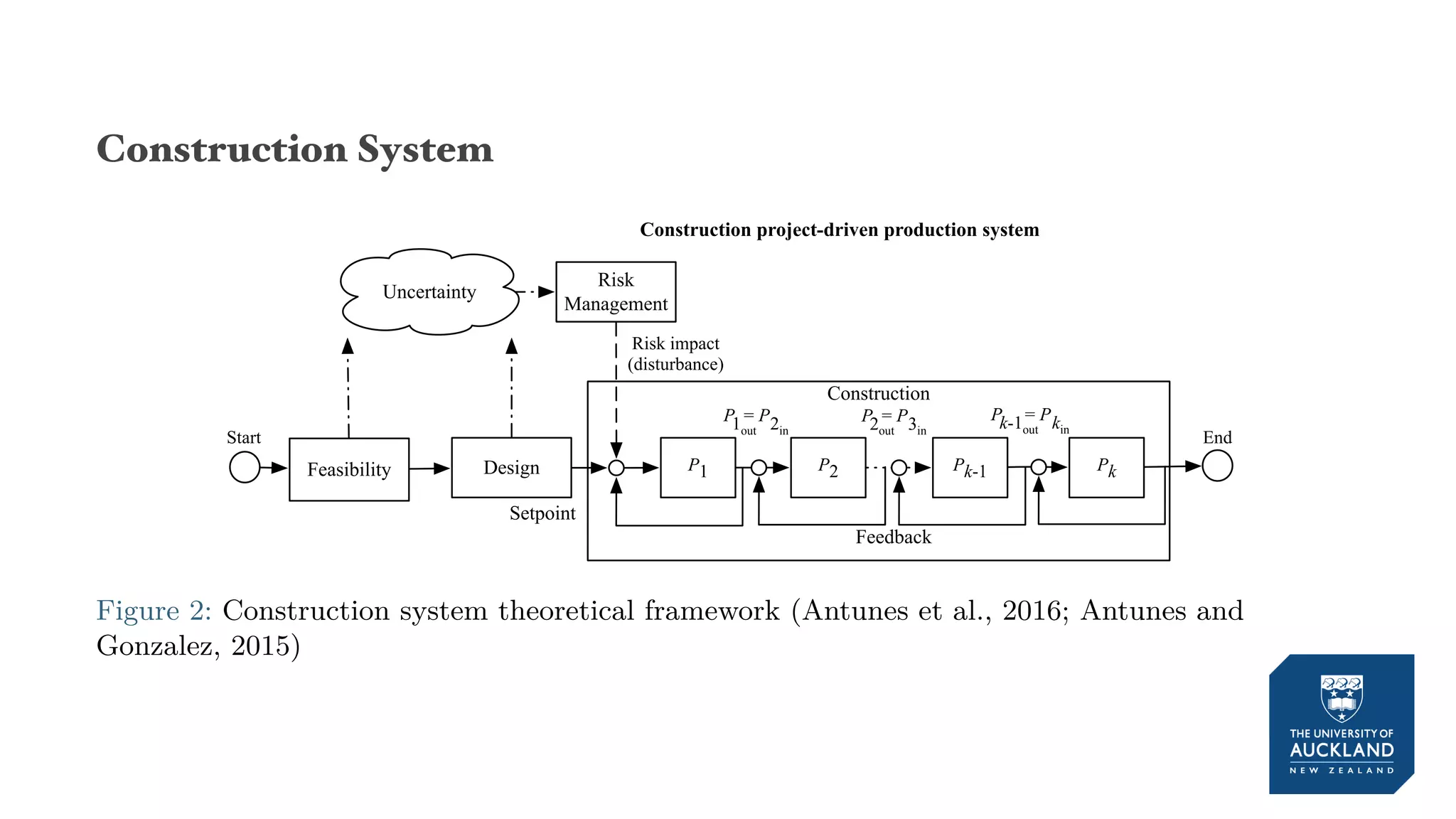
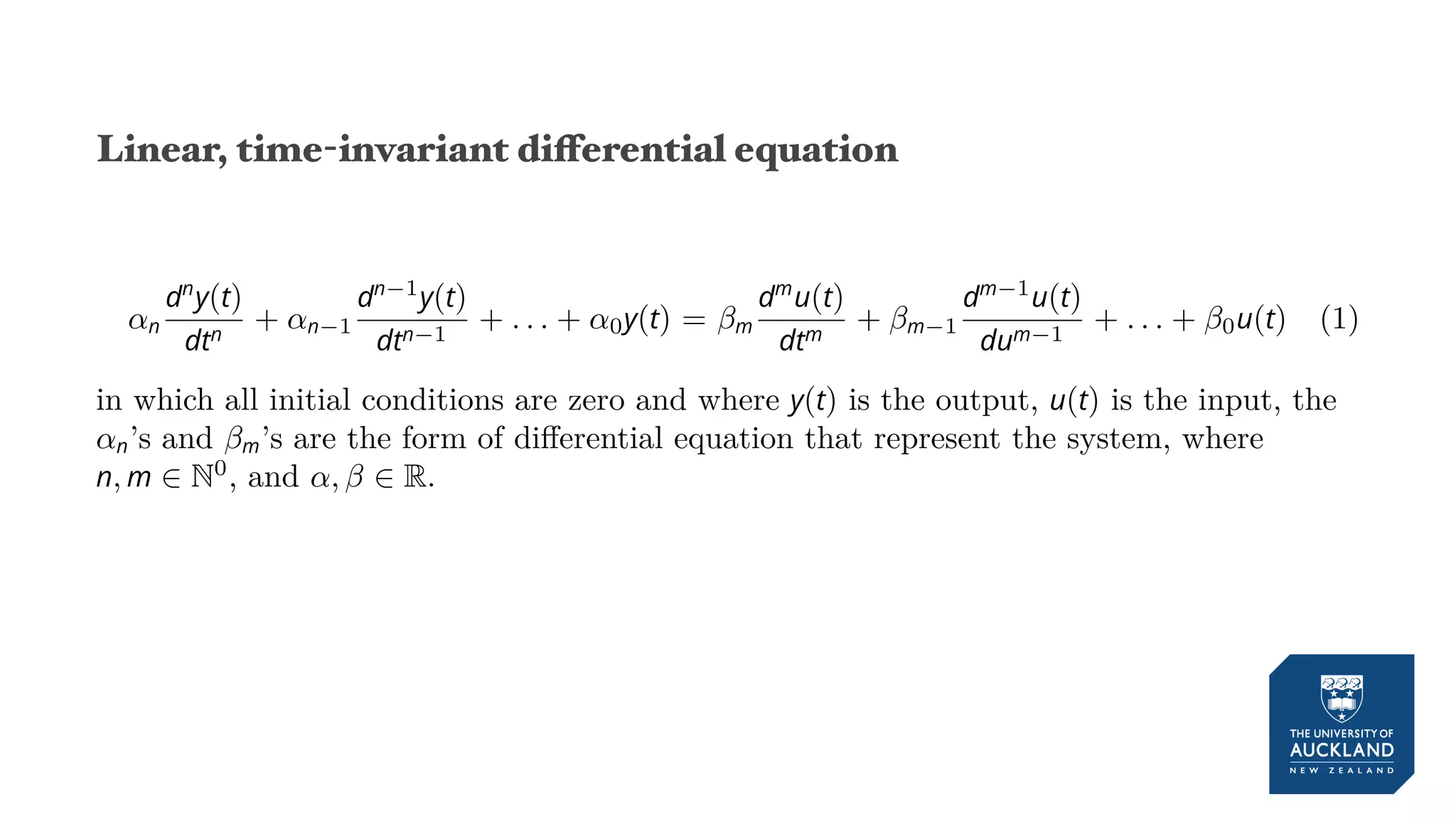
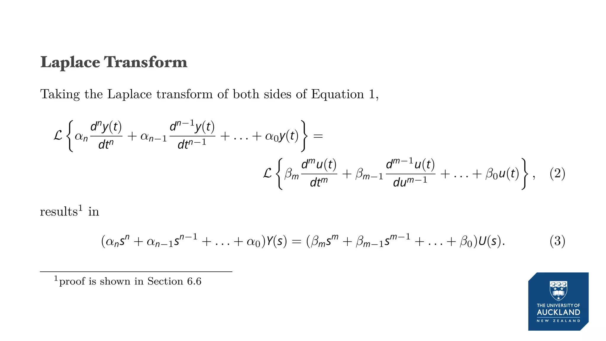
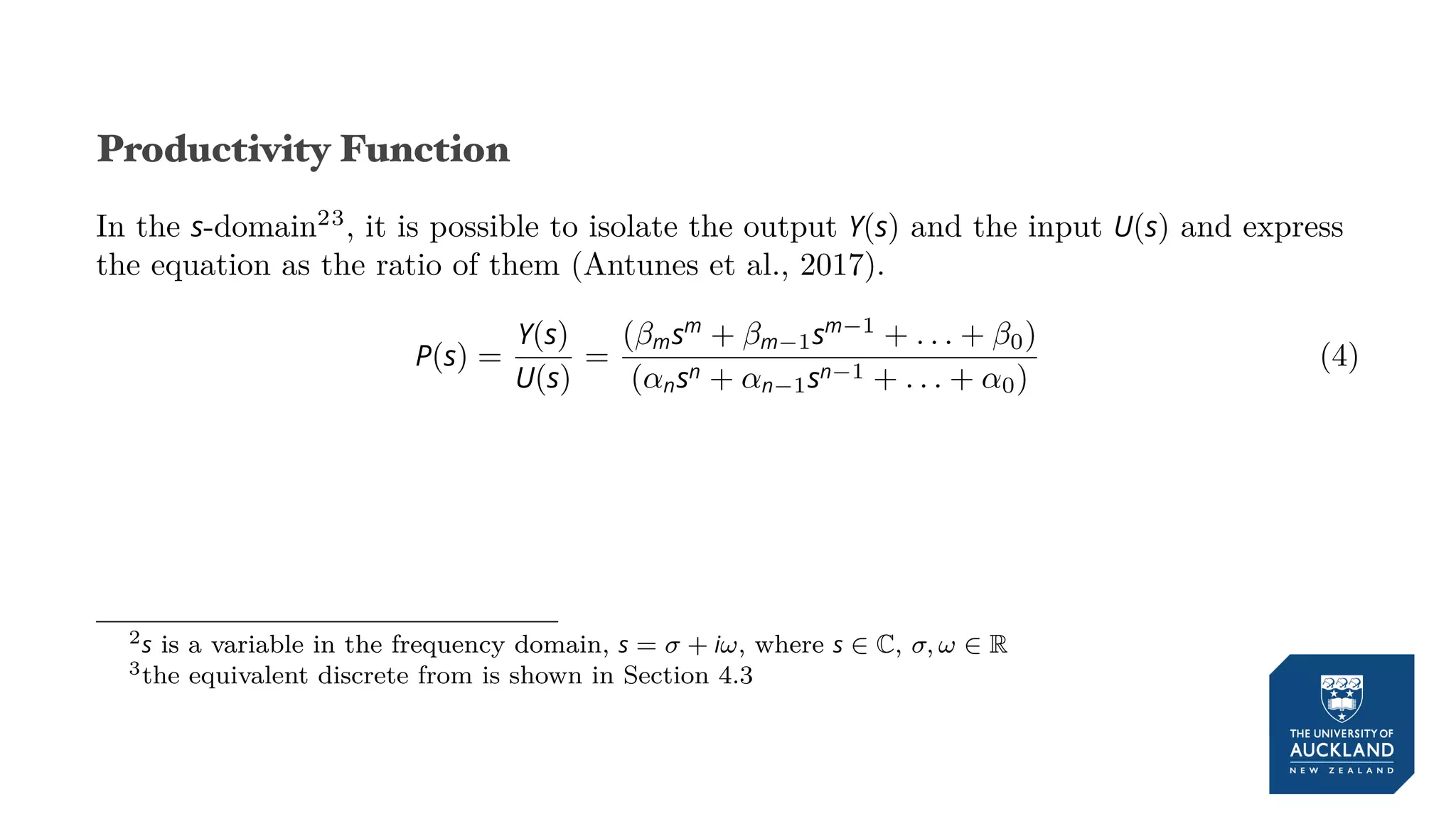
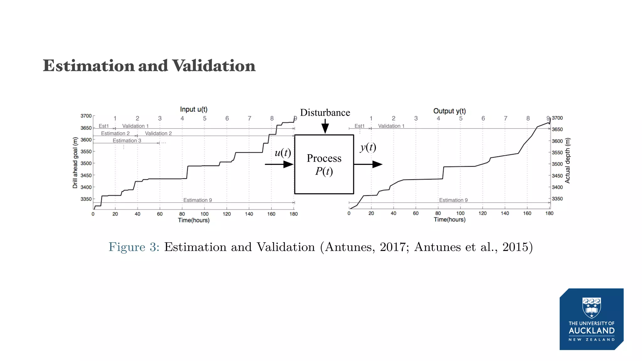
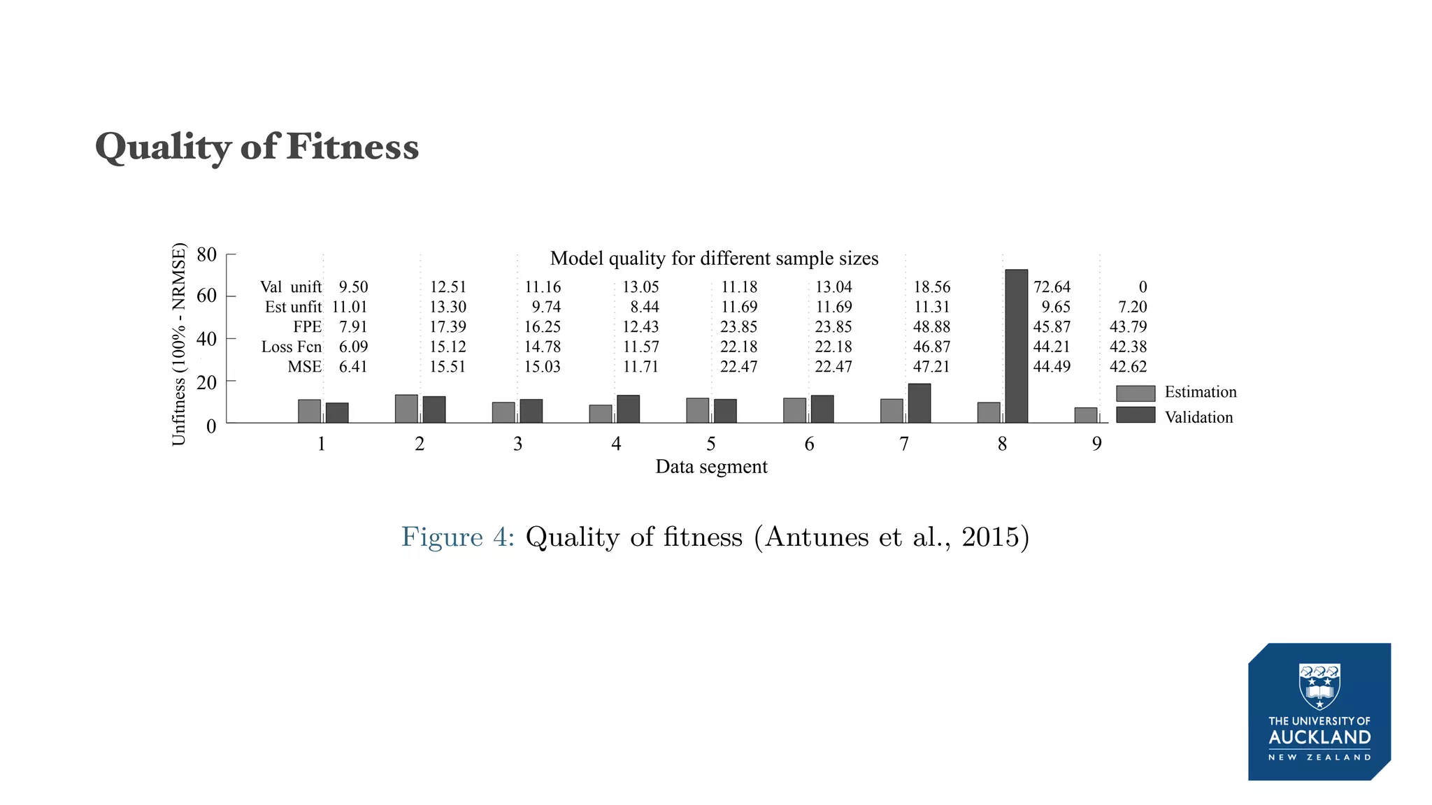
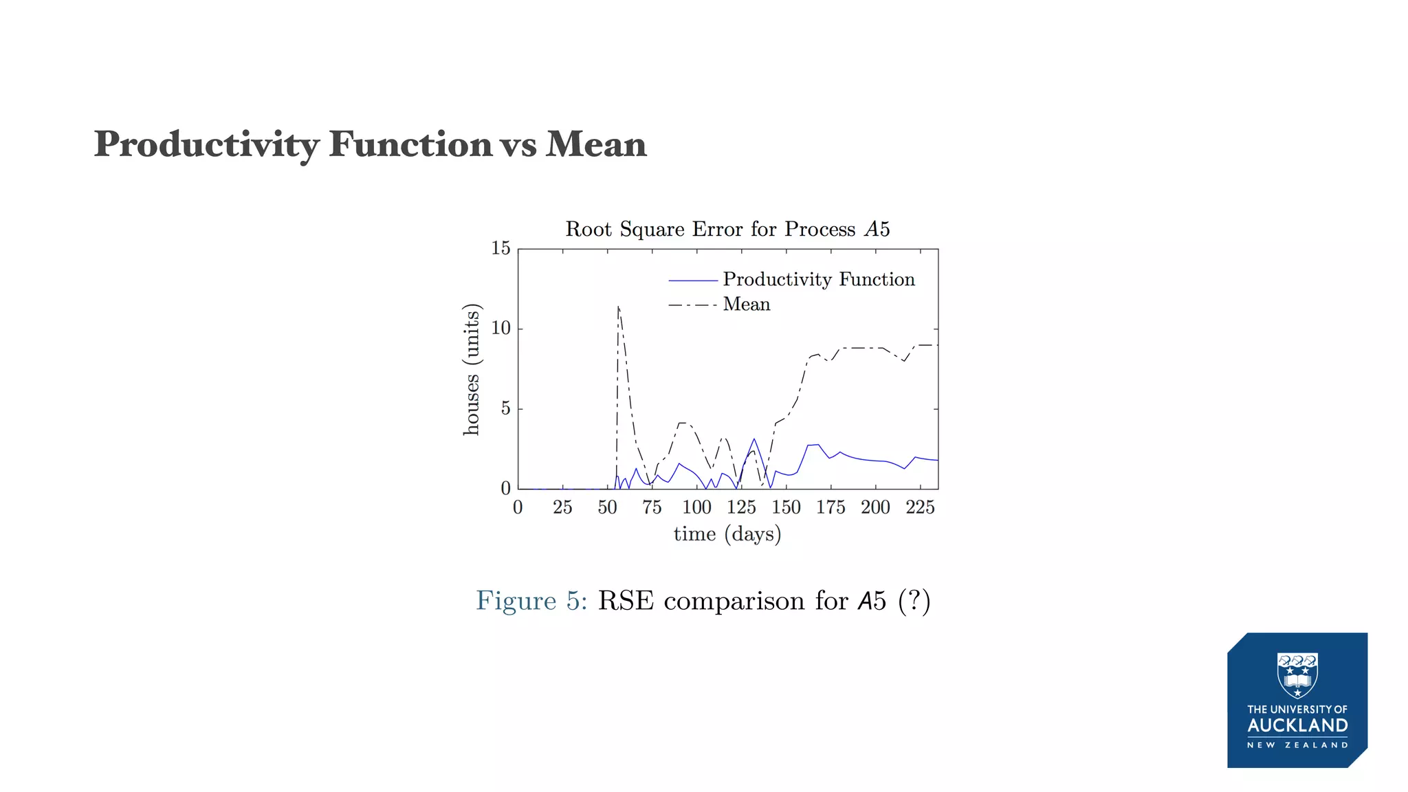
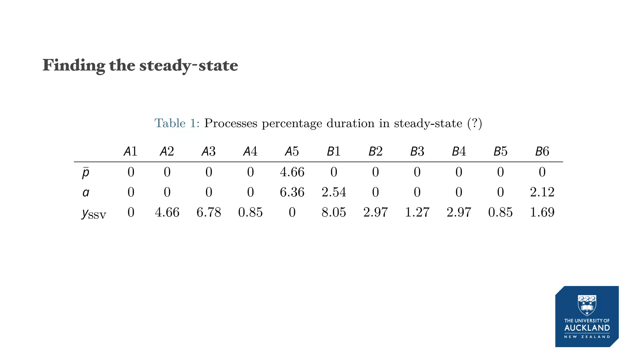
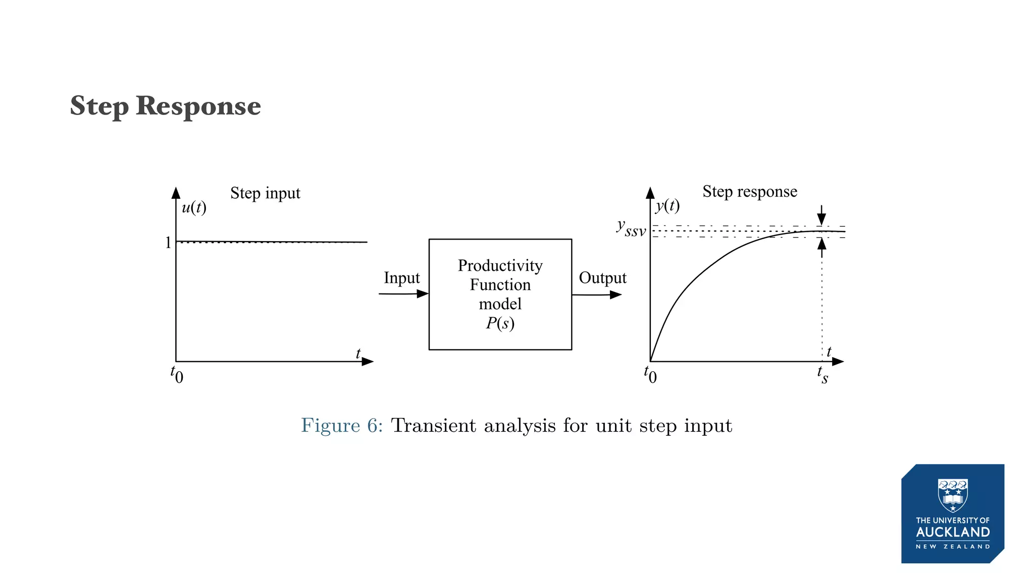
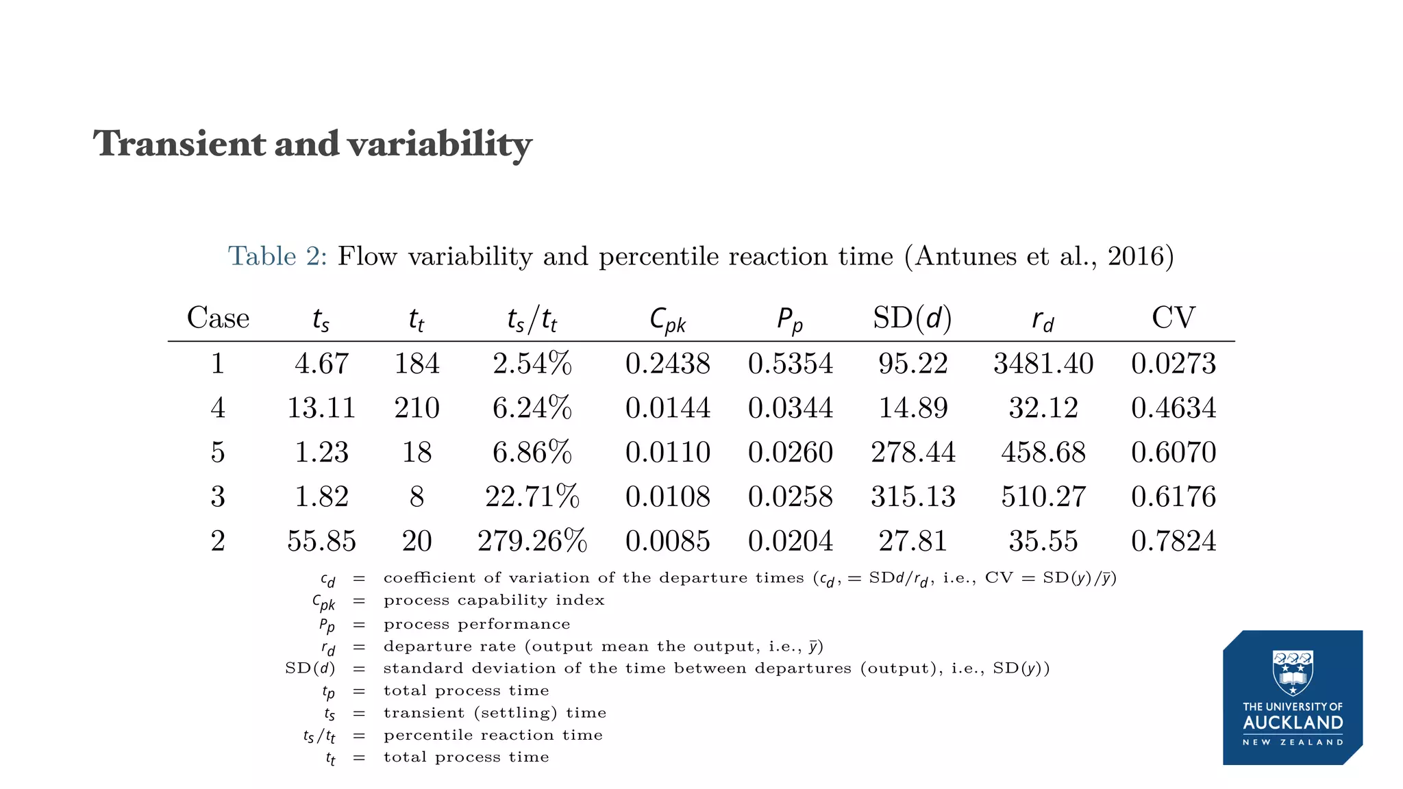
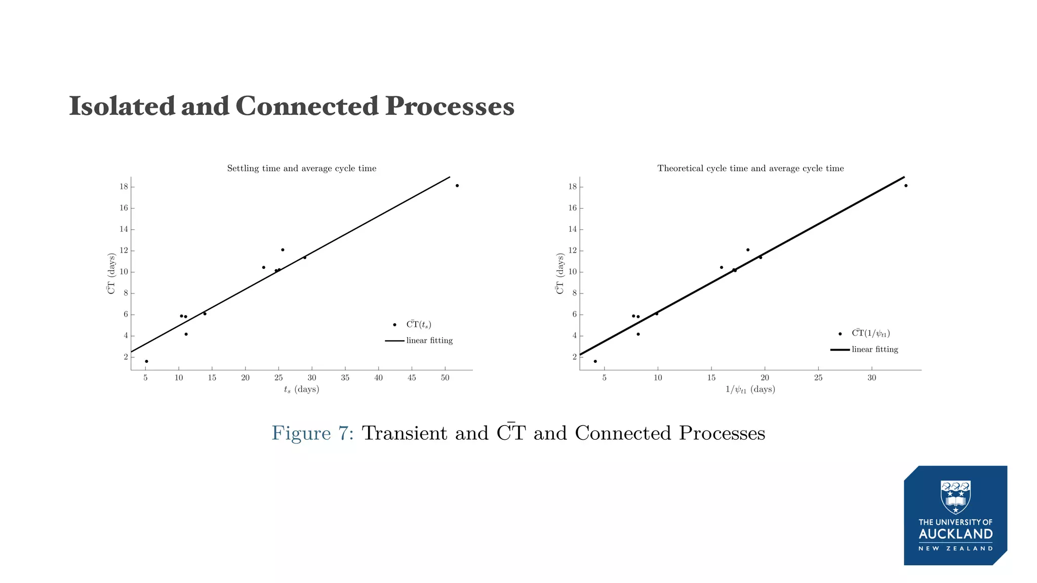
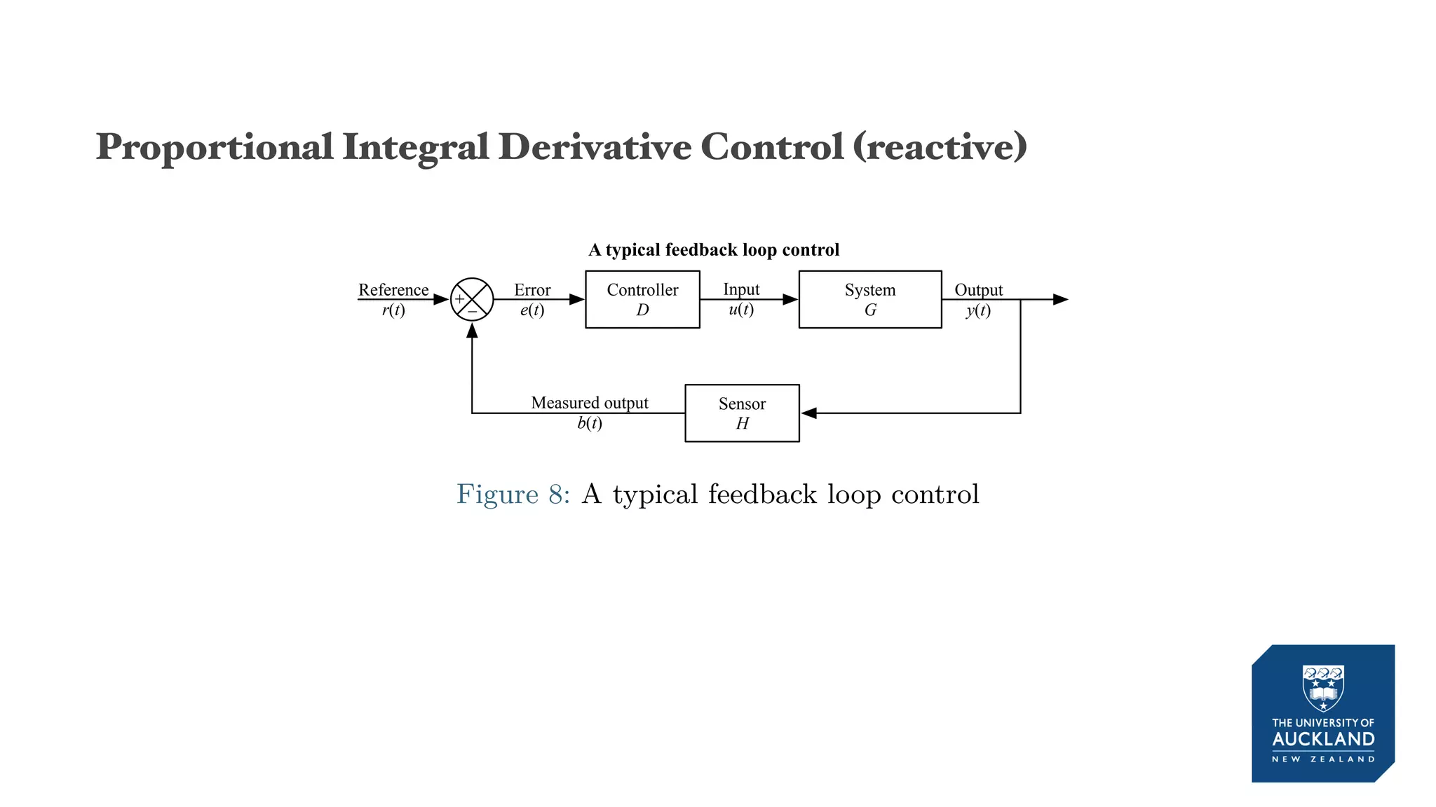
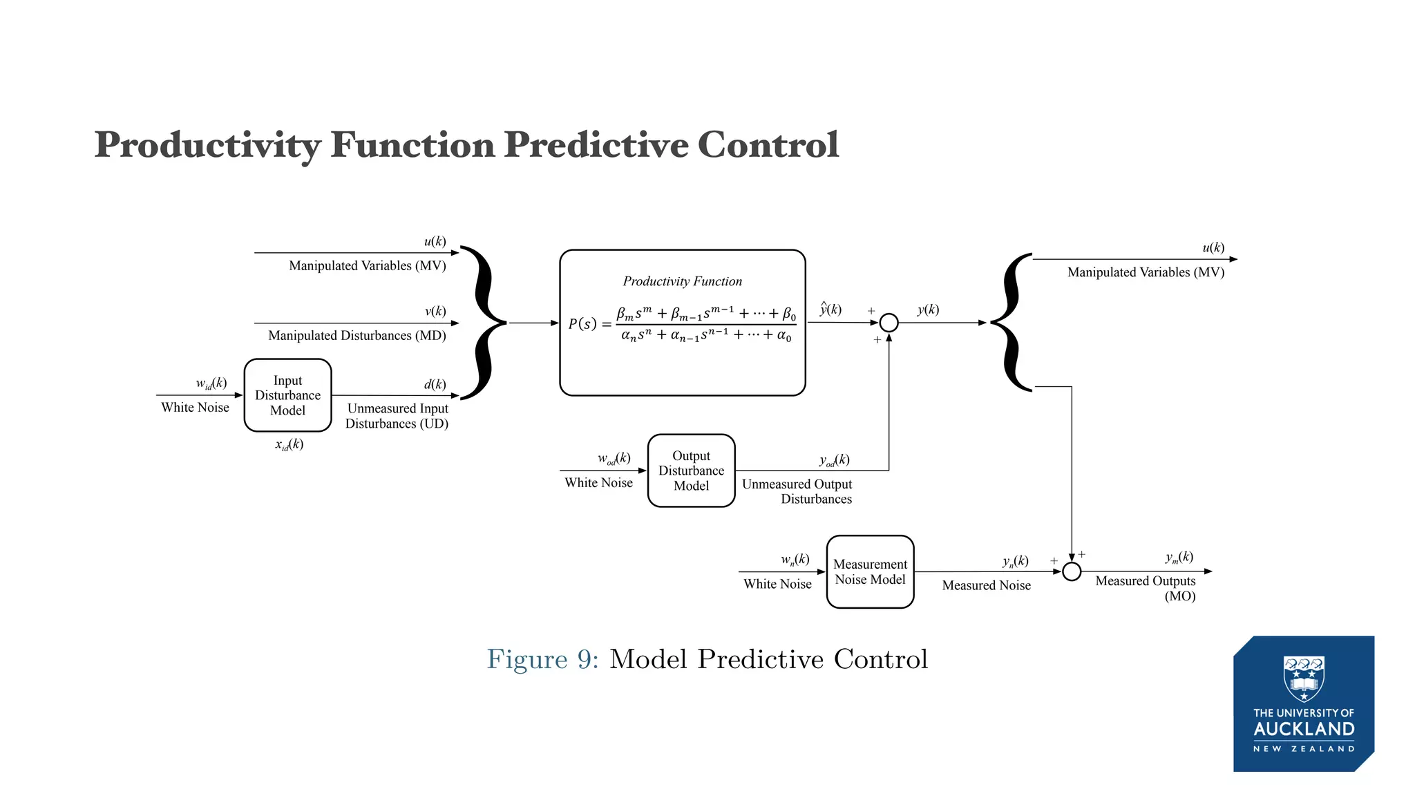
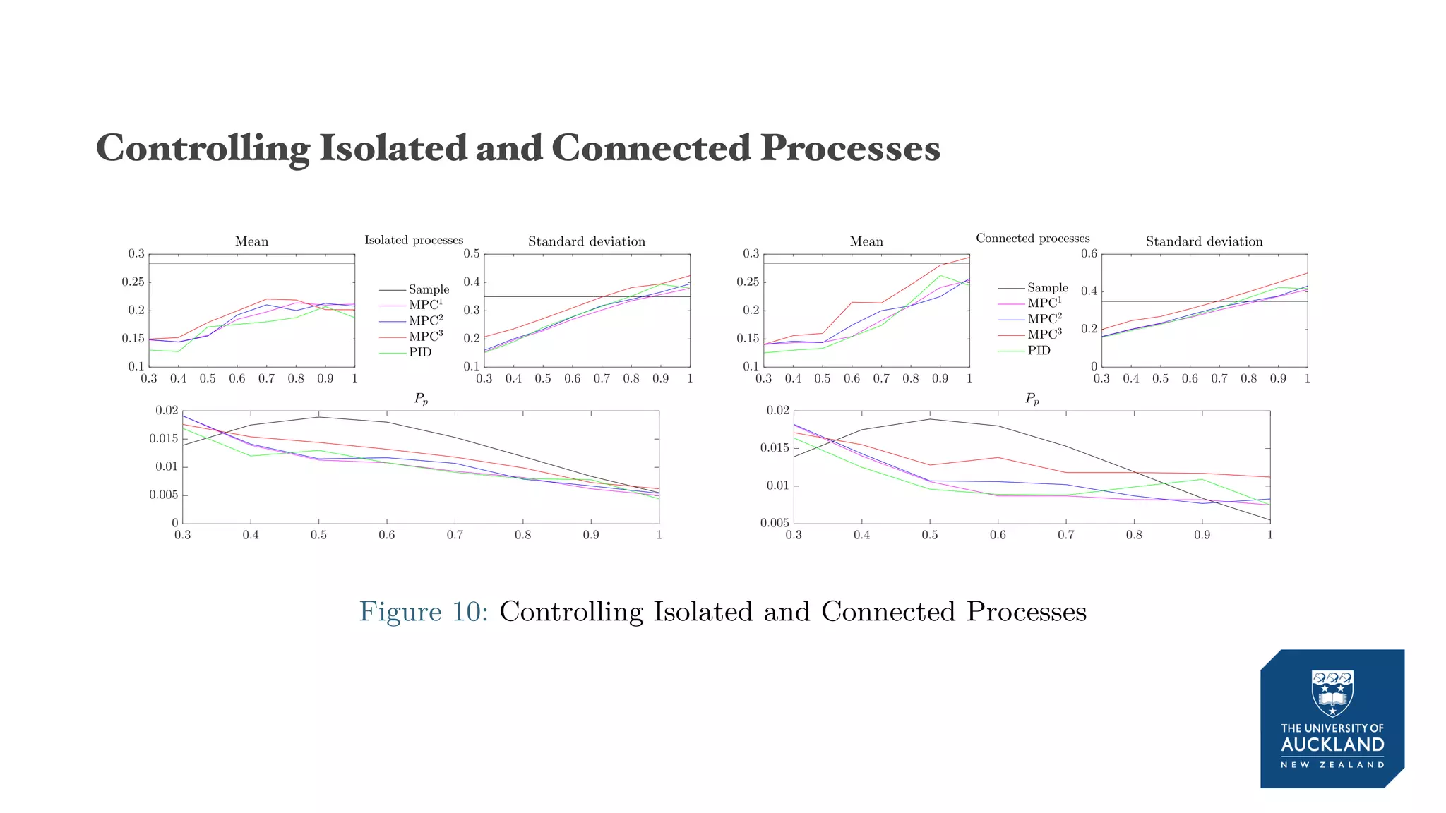
The document discusses a production model for repetitive processes in construction, focusing on the dynamics of project-driven systems. It emphasizes the importance of including transient states in modeling to enhance accuracy and provides methods for estimating productivity functions. Additionally, it highlights findings related to process variability and control methodologies while addressing limitations and future research directions.

1. Dynamics of project-driven systems
A production model for repetitive processes in construction
Ricardo Antunes
The University of Auckland
Department of Civil and Environmental Engineering
August 1, 2017

2. Outline
I - Research
II - A Production Model for Construction: A Theoretical Framework
III - Dynamics of production in Construction
Productivity Function
Estimation and Validation
Quality of Fitness
IV - Laws for production in project-driven processes in Construction
V - Control
VI - Conclusion
Findings
Limitations
Future Research

3. Research
Plan DoAct
Check
-setpoint error input output
Figure 1: PDCA Control Loop

4. Construction System
DesignFeasibility P1 P2 Pk-1 Pk
Setpoint
1out 2in
Start
Construction project-driven production system
Risk impact
(disturbance)
Risk
Management
Uncertainty
End
P = P 2out 3in
P = P k-1out kin
P = P
Construction
Feedback
Figure 2: Construction system theoretical framework (Antunes et al., 2016; Antunes and
Gonzalez, 2015)

5. Linear, time-invariant differential equation
αn
dn
y(t)
dtn
+ αn−1
dn−1
y(t)
dtn−1
+ . . . + α0y(t) = βm
dm
u(t)
dtm
+ βm−1
dm−1
u(t)
dum−1
+ . . . + β0u(t) (1)
in which all initial conditions are zero and where y(t) is the output, u(t) is the input, the
αn’s and βm’s are the form of differential equation that represent the system, where
n, m ∈ N0
, and α, β ∈ R.

6. Laplace Transform
Taking the Laplace transform of both sides of Equation 1,
L
{
αn
dn
y(t)
dtn
+ αn−1
dn−1
y(t)
dtn−1
+ . . . + α0y(t)
}
=
L
{
βm
dm
u(t)
dtm
+ βm−1
dm−1
u(t)
dum−1
+ . . . + β0u(t)
}
, (2)
results1
in
(αnsn
+ αn−1sn−1
+ . . . + α0)Y(s) = (βmsm
+ βm−1sm−1
+ . . . + β0)U(s). (3)
1proof is shown in Section 6.6

7. Productivity Function
In the s-domain23
, it is possible to isolate the output Y(s) and the input U(s) and express
the equation as the ratio of them (Antunes et al., 2017).
P(s) =
Y(s)
U(s)
=
(βmsm
+ βm−1sm−1
+ . . . + β0)
(αnsn + αn−1sn−1 + . . . + α0)
(4)
2s is a variable in the frequency domain, s = σ + iω, where s ∈ C, σ, ω ∈ R
3the equivalent discrete from is shown in Section 4.3

8. Estimation and Validation
u(t)
Process
P(t)
y(t)
Disturbance1 2 3 4 5 6 7 8 9 1 2 3 4 5 6 7 8 9
Est1 Validation 1
Estimation 2 Validation 2
Estimation 3 …
Est1 Validation 1
Estimation 9 Estimation 9
…
…
Actualdepth(m)
Figure 3: Estimation and Validation (Antunes, 2017; Antunes et al., 2015)

9. Quality of Fitness
Unfitness(100%–NRMSE)
Model quality for different sample sizes
Data segment
1
Unfitness(100%-NRMSE)
2 3 4 5 6 7 8 9
0
20
40
60
80
Estimation
Validation
9.50
11.01
7.91
6.09
6.41
12.51
13.30
17.39
15.12
15.51
11.16
9.74
16.25
14.78
15.03
13.05
8.44
12.43
11.57
11.71
11.18
11.69
23.85
22.18
22.47
13.04
11.69
23.85
22.18
22.47
18.56
11.31
48.88
46.87
47.21
72.64
9.65
45.87
44.21
44.49
0
7.20
43.79
42.38
42.62
Val unift
Est unfit
FPE
Loss Fcn
MSE
Figure 4: Quality of fitness (Antunes et al., 2015)

10. Productivity Function vs Mean
Figure 5: RSE comparison for A5 (?)

11. Finding the steady-state
Table 1: Processes percentage duration in steady-state (?)
A1 A2 A3 A4 A5 B1 B2 B3 B4 B5 B6
¯p 0 0 0 0 4.66 0 0 0 0 0 0
a 0 0 0 0 6.36 2.54 0 0 0 0 2.12
yssv 0 4.66 6.78 0.85 0 8.05 2.97 1.27 2.97 0.85 1.69

12. Step Response
Productivity
Function
model
P(s)
Input Output
Step input
u(t)
t
t0
1
Step response
y(t)
t
yssv
tst0
Figure 6: Transient analysis for unit step input

13. Transient and variability
Table 2: Flow variability and percentile reaction time (Antunes et al., 2016)
Case ts tt ts/tt Cpk Pp SD(d) rd CV
1 4.67 184 2.54% 0.2438 0.5354 95.22 3481.40 0.0273
4 13.11 210 6.24% 0.0144 0.0344 14.89 32.12 0.4634
5 1.23 18 6.86% 0.0110 0.0260 278.44 458.68 0.6070
3 1.82 8 22.71% 0.0108 0.0258 315.13 510.27 0.6176
2 55.85 20 279.26% 0.0085 0.0204 27.81 35.55 0.7824
cd = coefficient of variation of the departure times (cd, = SDd/rd, i.e., CV = SD(y)/¯y)
Cpk = process capability index
Pp = process performance
rd = departure rate (output mean the output, i.e., ¯y)
SD(d) = standard deviation of the time between departures (output), i.e., SD(y))
tp = total process time
ts = transient (settling) time
ts/tt = percentile reaction time
tt = total process time

14. Isolated and Connected Processes
5 10 15 20 25 30 35 40 45 50
ts (days)
2
4
6
8
10
12
14
16
18
¯CT(days)
Settling time and average cycle time
¯CT(ts)
linear fitting
5 10 15 20 25 30
1/ψt1 (days)
2
4
6
8
10
12
14
16
18
¯CT(days)
Theoretical cycle time and average cycle time
¯CT(1/ψt1)
linear fitting
Figure 7: Transient and ¯CT and Connected Processes

15. Proportional Integral Derivative Control (reactive)
Controller
D
+
System
G
Reference
r(t)
Output
y(t)
A typical feedback loop control
Sensor
H
_
Error
e(t)
Measured output
b(t)
Input
u(t)
Figure 8: A typical feedback loop control

16. Productivity Function Predictive Control
! " #
$%"%
& $%'("%'(
& ) & $*
+,", & +,'(",'( & ) & +*
Output
y(k)
Productivity Function
}
u(k)
Manipulated Variables (MV)
v(k)
Manipulated Disturbances (MD)
d(k)
Unmeasured Input
Disturbances (UD)
+
+
y(k)
{
u(k)
Manipulated Variables (MV)
Input
Disturbance
Model
wid(k)
White Noise
xid(k)
yod(k)
Unmeasured Output
Disturbances
Output
Disturbance
Model
wod(k)
White Noise
+yn(k)
Measured Noise
Measurement
Noise Model
wn(k)
White Noise
+ ym(k)
Measured Outputs
(MO)
^
Figure 9: Model Predictive Control

17. Controlling Isolated and Connected Processes
0.3 0.4 0.5 0.6 0.7 0.8 0.9 1
0.1
0.15
0.2
0.25
0.3
Mean
Sample
MPC1
MPC2
MPC3
PID
Isolated processes
0.3 0.4 0.5 0.6 0.7 0.8 0.9 1
0.1
0.2
0.3
0.4
0.5
Standard deviation
0.3 0.4 0.5 0.6 0.7 0.8 0.9 1
0
0.005
0.01
0.015
0.02
Pp
0.3 0.4 0.5 0.6 0.7 0.8 0.9 1
0.1
0.15
0.2
0.25
0.3
Mean
Sample
MPC1
MPC2
MPC3
PID
Connected processes
0.3 0.4 0.5 0.6 0.7 0.8 0.9 1
0
0.2
0.4
0.6
Standard deviation
0.3 0.4 0.5 0.6 0.7 0.8 0.9 1
0.005
0.01
0.015
0.02
Pp
Figure 10: Controlling Isolated and Connected Processes

18. Findings
1. There is transient state in project-driven construction processes
2. This transient can be measured
3. Including the transient on the modeling yields in more accurate models
4. Only 5 samples are required to estimate a Productivity Function model.
5. An input/output correlation higher than 60% is required.
6. A qualify of fitness higher than steady-state approaches is enough
7. Higher the transient time, higher the variability
8. Higher the transient time, higher the average cycle time
9. Equation for capacity P(0) but perform at capacity is challenging
10. Predictive control rather than reactive control

19. Limitations
1. Exploratory stage
2. No case illustrating unsteady state
3. Requires an input and output data
4. Model accuracy cannot be evaluated until some data has been produced
5. Some concepts are unfamiliar to general construction managers
6. One transient curve to represent all

20. What next?
• Productivity Function and Learning Curve models
• Process’ variability using Bode-plots
• Simulated Risk Impact: extreme shock, wavelets (?, Fig.4)…
• Multi-input-multi-output modeling and case analyses
• Nonlinear models (also to be compared with multi variable Learning Curve models)

21. Bibliography
Antunes, R. Offshore rig, drilling well, Brazil 2013, v1, 2017. URL https://data.mendeley.com/datasets/xn88z63ghs/1.
Antunes, R., González, V. A., Walsh, K., Gonzalez, V. A., and Walsh, K. Identification of repetitive processes at steady- and
unsteady-state: Transfer function. In 23rd Annual Conference of the International Group for Lean Construction, pages 793–802,
Perth, Australia, 2015. ISBN 9780987455796. doi: 10.13140/RG.2.1.4193.7364. URL
http://iglc.net/papers/Details/1194http://www.iglc.net/papers/details/1194.
Antunes, R., González, V., and Walsh, K. Quicker reaction, lower variability: The effect of transient time in flow variability of
project-driven production. In 24th Annual Conference of the International Group for Lean Construction, pages sect.1 pp. 73–82,
Boston, MA, 2016. URL http://iglc.net/papers/Details/1332.
Antunes, R., González, V. A., Walsh, K., and Rojas, O. Dynamics of Project-Driven Production Systems in Construction:
Productivity Function. Journal of Computing in Civil Engineering, 31(5):17, 2017. ISSN 0887-3801. doi:
10.1061/(ASCE)CP.1943-5487.0000703. URL http://ascelibrary.org/doi/10.1061/{%}28ASCE{%}29CP.1943-5487.0000703.
Antunes, R. M. S. and Gonzalez, V. A production model for construction: A theoretical framework. In Building a Better New
Zealand, pages 223–233, Porirua, New Zealand, 2015. Branz Ltd. ISBN 978-1-927258-42-2. URL
http://www.buildingabetternewzealand.co.nz/cms{_}show{_}download.php?id=202.