Downloaded 249 times

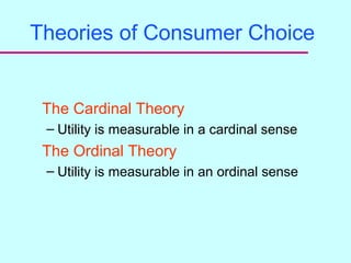


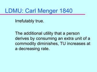


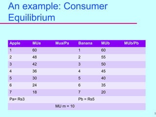
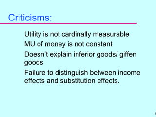


Consumer theory helps understand how individuals make choices given limited budgets to maximize satisfaction or utility. It assumes consumers are rational and want to maximize utility subject to budget constraints. There are two main approaches - the cardinal and ordinal theories. The cardinal theory assumes utility is quantitatively measurable while the ordinal theory only requires preferences can be ranked. Both use concepts like total utility, marginal utility, indifference curves, and budget constraints to model consumer choice and derive the downward sloping demand curve. The law of diminishing marginal utility states that as consumption of a good increases, the marginal utility from each additional unit decreases. This forms the basis for consumer demand curves and many economic implications.