Downloaded 65 times
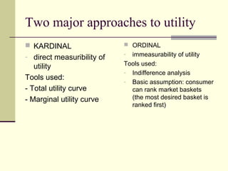


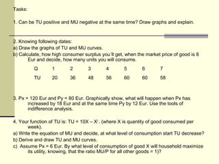

1. There are two approaches to analyzing utility - the cardinal and ordinal approaches. The cardinal approach measures utility directly while the ordinal only ranks preferences. 2. The law of diminishing marginal utility states that as consumption of a good increases, the marginal utility of each additional unit decreases. 3. A consumer will purchase goods up to the point where the marginal utility per dollar spent is equal across all goods, reaching equilibrium. This is known as the equimarginal principle. 4. Indifference curves show combinations of goods that provide equal utility. The budget constraint shows affordable combinations. The optimal choice is where an indifference curve is tangent to


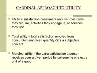
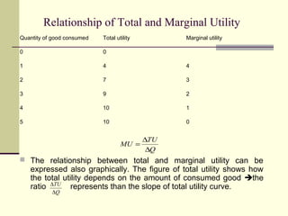
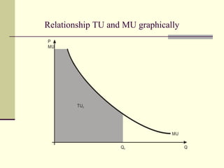
![725Actual Session 126 (5) [Autosaved].pptx](https://cdn.slidesharecdn.com/ss_thumbnails/725actualsession1265autosaved-220908132926-94ed533e-thumbnail.jpg?width=640&height=640&fit=bounds)


