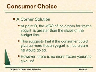
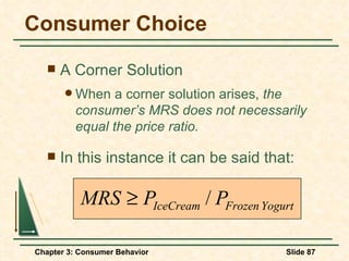
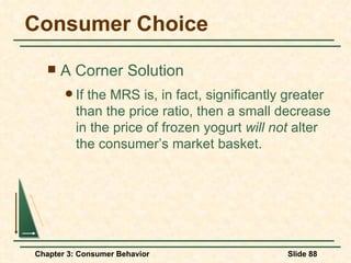
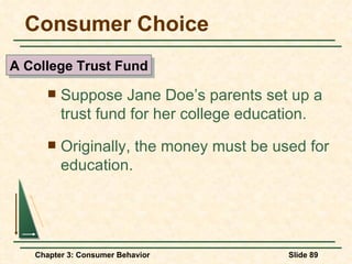
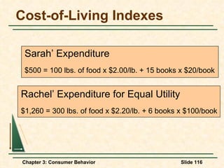
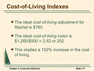
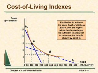
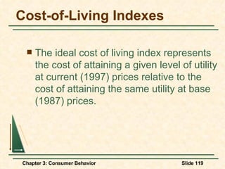
This document summarizes key topics in consumer behavior including:
1) It outlines the three steps in studying consumer behavior: understanding consumer preferences, budget constraints, and how preferences and constraints determine consumer choices.
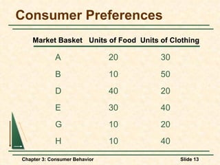
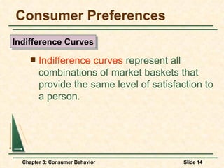
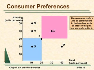
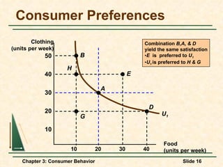
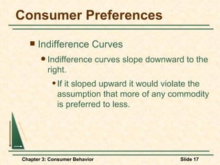
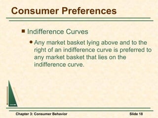
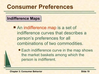
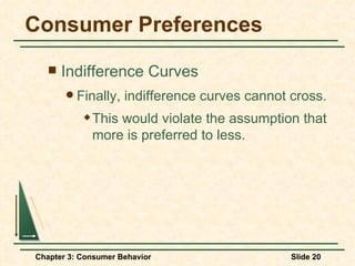
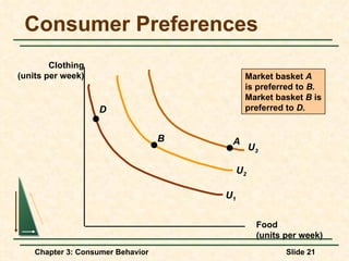
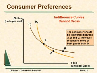
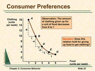
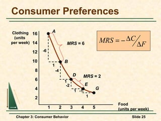
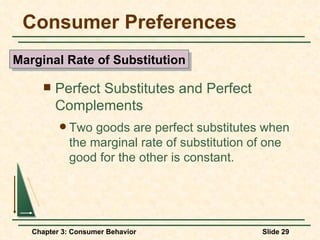
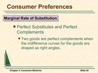
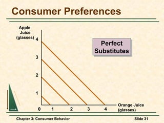
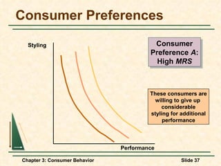
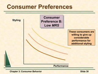
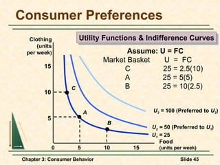
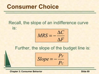
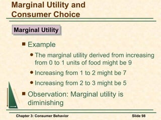
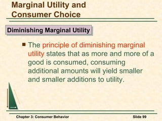
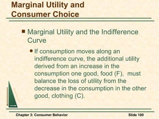
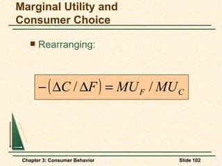
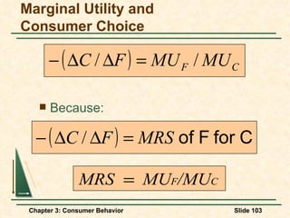
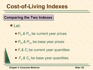
2) It discusses indifference curves and how they represent combinations of goods that provide equal satisfaction. The slope of indifference curves illustrates the marginal rate of substitution.
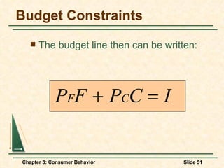
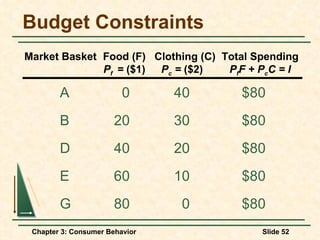
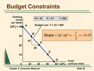
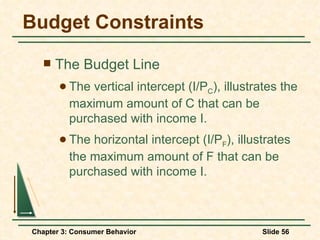
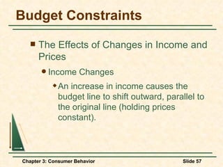
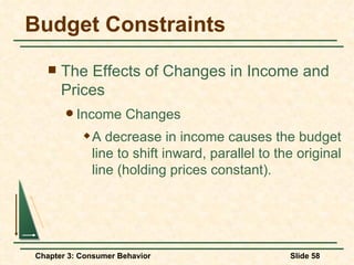
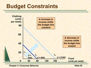
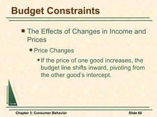
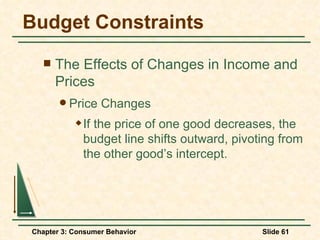
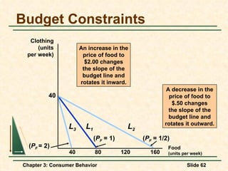
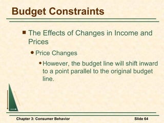
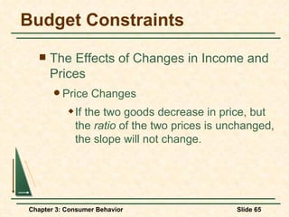
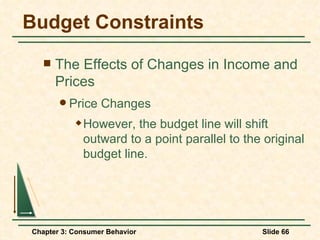
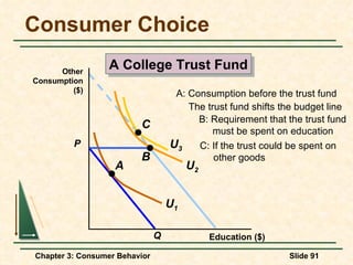
3) It explains budget constraints and how the budget line represents all combinations of goods that can be purchased given prices and income. Changes in income and prices affect the position of the budget line.
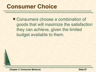
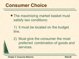
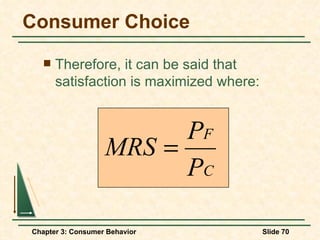
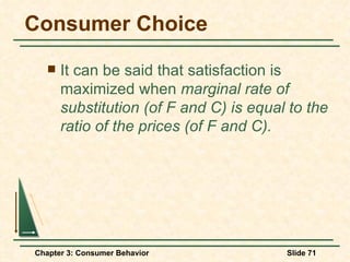
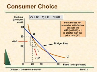
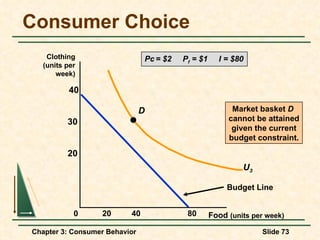
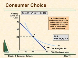
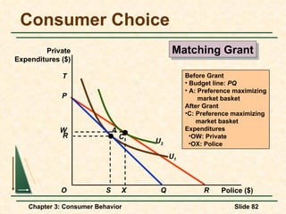
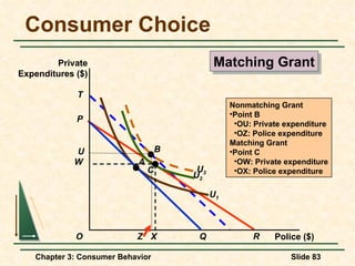
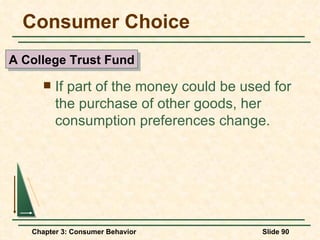
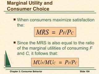
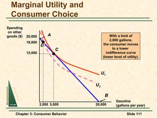
4) Consumer choice is where the budget line is tangent to the highest indifference curve, indicating preferences are maximized subject to the budget constraint.


![indifference curve analysis [Autosaved].pptx](https://cdn.slidesharecdn.com/ss_thumbnails/indifferencecurveanalysisautosaved-230212040058-9caa8b7a-thumbnail.jpg?width=640&height=640&fit=bounds)
![[PERT-3] Consumer Behaviour.pdf](https://cdn.slidesharecdn.com/ss_thumbnails/pert-3consumerbehaviour-231017015937-da9d2839-thumbnail.jpg?width=640&height=640&fit=bounds)


