Comparison of Distance Transform Based Features

Satish Kumar. Int. Journal of Engineering Research and Applications www.ijera.com
ISSN: 2248-9622, Vol. 6, Issue 4, (Part - 7) April 2016, pp.63-66
www.ijera.com 63 | P a g e
Comparison of Distance Transform Based Features
Satish Kumar
Panjab University SSG Regional Centre, Hoshiarpur, Punjab(India)
ABSTRACT
The distance transform based features are widely used in pattern recognition applications. A distance transform
assigns to each background pixel in a binary image a value equal to its distance to the nearest foreground pixel
according to a defined metric. Among these metrics the Chessboard, Euclidean, Chamfer and City-block are
popular. The role of a feature extraction method is quite important in pattern recognition applications. Before
applying a feature, it is essential to judge its performance on the given applications. In this research work, a
study on the performance of above mentioned distance transform based features is made. We have conducted
experiments with 500 hand-printed characters/class and the study has been performed on 43 classes. The
classifiers used are k-NN, MLP, SVM and PNN.
Keywords – Characters, Devanagari, Distance Transform, Hand-printed, Recognition
I. INTRODUCTION
A recognition system works in various stages such
as scanning, preprocessing, feature extraction,
classification and post processing. In a typical
pattern recognition problems the feature extraction
phase plays an important role as some essential
properties of the images are extracted in this phase
that is important for taking a classification decision.
If we look at the hand-printed character images
which are contributed by different writers having
varying writing styles. There is a lot of variability in
the hand-printed images within each class that is not
easy to handle. The properties used to segregate the
characters must possess small intra-class variability
and large inter-class separation capability.
The distance transform (DT) is a technique in
which the distance relationships among the pixels of
an image are used to obtain a feature map. It
converts a binary image into a gray level distance
map (DM). The DT algorithm proposed by
Rosenfeld et al[1] is earliest. The DT based features
have been used by Smith et al [3], Koύacs et al [4]
and Oh et al[5] for handwritten recognition and Negi
et al [78] for machine-printed Telugu character
recognition. In [4], the L1 norm is used as distance
metric to compute DT of a binary image where
distance map is computed from a 32×32 image and
subsequently it is sub-sampled to 8×8. In [3],
Hamming distance, pixel distance and pen-stroke are
used as a distance measure. In [5] its performance is
compared with other features on English capital
letters, English numerals and Hangul characters and
Manhattan distance metric is used for this purpose.
In this case distance map is computed from 16×16
binary image giving 256 features.
Selecting a best technique for a particular
application is a daunting task. One has to
exhaustively study the literature, implement them
and observe their performance. Obviously this is a
big task. As far as feature extraction stage is
concerned, Govindan et al[9] classified the various
features in three categories i.e. statistical, structural
and global transforms and series expansion. Each
category has its pros and cons in terms of
computational speed, computational complicacy and
accuracy. The distance transform based features are
statistical features.
The paper is arranged as follows: Section II
covers Distance Transform, Section III covers
Feature Extraction, Section IV covers Experimental
Results, Section V covers Discussion and
Conclusion.
II. DISTANCE TRANSFORM
The A distance transform assigns to each white
pixel (background) of a binary image a value equal
to its distance to the nearest black pixels
(foreground) according to a defined metric. A new
image, which has same size as that of an original
image, is created using distance transform and this
image is called as distance map (DM). In DM each
background pixel has some value whereas each
foreground pixel has 0 value. The distance map of
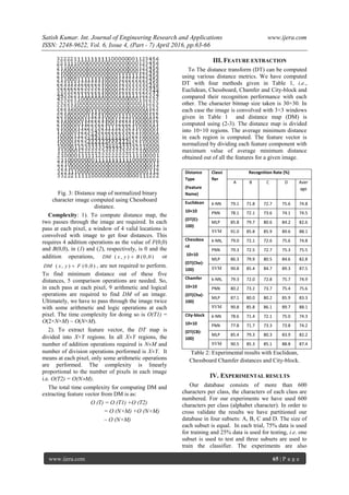
3030 binary image (Fig. 2) computed using
Chessboard distance as a metric is given in Fig. 3.
Borgefors[2] presented the Chamfer distance
algorithm(CDA) that efficiently and accurately
calculates the DT of 2 dimensional images[5,6]. It
works in two passes. Initially the distance map as
well as the character image is padded with two extra
rows (one each on top and bottom) and two extra
RESEARCH ARTICLE OPEN ACCESS

columns (one each on left and right). These extra
pixels are treated as background pixels in a given
image. The distance map is initialized as:


 

Otherwisev
blackeiyxIif
yxDM
..1),(0
),(
(1)
Where v is infinite or we may choose a
sufficiently large value.
Pass 1: In this pass distance map is scanned in
forward direction, i.e., top to bottom and left to right.
Minimum distance for each position of the distance
map is computed using a 3×3 forward mask F which
is given in Figure 1(a).
a) b)
Fig. 1 : a) Forward mask F ; b) Backward
mask B.
For a given location (x,y) of distance map (DM),
the minimum distance is computed as:















)0,0(),(
),0,1(),1(
),1,1()1,1(
),1,0()1,(
),1,1()1,1(
min),(
FyxDM
FyxDM
FyxDM
FyxDM
FyxDM
yxDM
(2)
Pass 2: In this pass distance map is scanned in
backward direction. Minimum distance for each
position of the distance map is computed using a
3×3 backward mask B which is given in Fig. 1(b).
For a given location (x,y) of distance map (DM), the
minimum distance is computed as:















)0,0(),(
),1,1()1,1(
),1,0()1,(
),1,1()1,1(
),0,1(),1(
min),(
ByxDM
ByxDM
ByxDM
ByxDM
ByxDM
yxDM
(3)
The values of „#‟ and „*‟ in both masks depend
upon the type of distance metric used. The value of
‘o’ is zero in both masks and `–` represents a point
that is not to be used in computation. The various
33 masks used during forward and backward
scanning depends upon the type of distance metric
used and some of these masks are given in Table 1.
TABLE 1: Some Metric Distances and Their
Corresponding Forward and Backward Masks.
Distance
Metric
Chamfer
Distance
Euclidean
Distance
Chessboar
d
Distance
City-
block
Distance
Forward Scan
4 3 4
3 o -
- - -
2 1 2
1 o -
- - -
1 1 1
1 o -
- - -
- 1 -
1 o -
- - -
Backward Scan
- - -
- o 3
4 3 4
- - -
- o 1
2 1 2
- - -
- o 1
1 1 1
- - -
- o 1
- 1 -
Fig. 2: A normalized binary character image.

Fig. 3: Distance map of normalized binary
character image computed using Chessboard
distance.
Complexity: 1). To compute distance map, the
two passes through the image are required. In each
pass at each pixel, a window of 4 valid locations is
convolved with image to get four distances. This
requires 4 addition operations as the value of F(0,0)
and B(0,0), in (1) and (2), respectively, is 0 and the
addition operations, )0,0(),( ByxDM  or
)0,0(),( FyxDM  , are not required to perform.
To find minimum distance out of these five
distances, 5 comparison operations are needed. So,
in each pass at each pixel, 9 arithmetic and logical
operations are required to find DM of an image.
Ultimately, we have to pass through the image twice
with some arithmetic and logic operations at each
pixel. The time complexity for doing so is O(T1) =
O(2×N×M) ~ O(N×M).
2). To extract feature vector, the DT map is
divided into X×Y regions. In all XY regions, the
number of addition operations required is NM and
number of division operations performed is XY. It
means at each pixel, only some arithmetic operations
are performed. The complexity is linearly
proportional to the number of pixels in each image
i.e. O(T2) = O(NM).
The total time complexity for computing DM and
extracting feature vector from DM is as:
O (T) = O (T1) +O (T2)
= O (N×M) +O (N×M)
~ O (N×M)
III. FEATURE EXTRACTION
To The distance transform (DT) can be computed
using various distance metrics. We have computed
DT with four methods given in Table 1, i.e.,
Euclidean, Chessboard, Chamfer and City-block and
compared their recognition performance with each
other. The character bitmap size taken is 30×30. In
each case the image is convolved with 3×3 windows
given in Table 1 and distance map (DM) is
computed using (2-3). The distance map is divided
into 10×10 regions. The average minimum distance
in each region is computed. The feature vector is
normalized by dividing each feature component with
maximum value of average minimum distance
obtained out of all the features for a given image.
Distance
Type
(Feature
Name)
Classi
fier
Recognition Rate (%)
A B C D Aver
age
Euclidean
10×10
(DT(E)-
100)
k-NN 79.1 71.8 72.7 75.6 74.8
PNN 78.1 72.1 73.6 74.1 74.5
MLP 85.8 79.7 80.6 84.2 82.6
SVM 91.0 85.8 85.9 89.6 88.1
Chessboa
rd
10×10
(DT(Che)-
100)
k-NN, 79.0 72.1 72.6 75.6 74.8
PNN 79.3 72.5 72.7 75.3 75.5
MLP 86.3 79.9 80.5 84.6 82.8
SVM 90.8 85.4 84.7 89.3 87.5
Chamfer
10×10
(DT(Cha)-
100)
k-NN, 79.3 72.0 72.8 75.7 74.9
PNN 80.2 73.2 73.7 75.4 75.6
MLP 87.1 80.0 80.2 85.9 83.3
SVM 90.8 85.8 86.1 89.7 88.1
City-block
10×10
(DT(CB)-
100)
k-NN 78.6 71.4 72.1 75.0 74.3
PNN 77.8 71.7 73.3 73.8 74.2
MLP 85.4 79.3 80.3 83.9 82.2
SVM 90.5 85.3 85.1 88.8 87.4
Table 2: Experimental results with Euclidean,
Chessboard Chamfer distances and City-block.
IV. EXPERIMENTAL RESULTS
Our database consists of more than 600
characters per class, the characters of each class are
numbered. For our experiments we have used 600
characters per class (alphabet character). In order to
cross validate the results we have partitioned our
database in four subsets: A, B, C and D. The size of
each subset is equal. In each trial, 75% data is used
for training and 25% data is used for testing, i.e. one
subset is used to test and three subsets are used to
train the classifier. The experiments are also

conducted by partitioning the distance map into 4×4,
6×6 and 8×8 regions, but the recognition rates
recoded are low as compared to the recognition rates
for 10×10 given in Table 2.
V. DISCUSSION AND CONCLUSION
The following can be concluded from the results:
1). The results of Table 2 clearly predict the
superiority of Chamfer and Euclidean distances over
Chessboard.
2). Performance of Chamfer and Euclidean is neck
to neck in case of SVM whereas Chamfer is more
than Euclidean on PNN, k-NN and MLP.
3). Performance of Chessboard and city-block is
neck to neck in case of SVM whereas Chessboard is
more than city-block on PNN, k-NN and MLP.
4) The City-block is performing least as compared
to other classifiers on all classifiers.
5) The k-NN and PNN are performing neck to
neck.
The better recognition rates in these two cases are
due to the fact that the values of constants „*‟ and
„#‟ taken in forward and backward windows, in both
these cases, are different as compared to Chessboard
where these values are same. The maximum
recognition rate achieved with SVM classifier is
88.1 % and with MLP classifier is 83.3%. Both
Chamfer and Euclidean distance metric give same
results with SVM. However, their results with MLP
are different. If we want to use MLP then Chamfer
distance is better as compared to Euclidean distance.
Fig. 4: Recognition performance of various distance
metrics.
Fig. 5: Recognition performance of various
classifiers.
REFERENCES
[1] A. Rosenfeld and J. L. Pfaltz, “Distance
Functions on Digital Pictures”, Pattern
Recognition, Vol. 1(1), 1968, 33-61(1968).
[2] G. Borgefors, “Distance Transformations in
Digital Images”, Computer Vision, Graphics
and Image Processing, 34, 1986, 344-371.
[3] S. J. Smith, M. O. Bourgoin, K. Sims and
H.L. Voorhees, “Handwritten Character
Classification using Nearest Neighbor in
Large Database”, IEEE Transactions on
Pattern Analysis and Machine Intelligence,
16(9), 1994, 915-919.
[4] Zs. M. Kovics and R. Guerrieri, “Massively-
Parallel Handwritten Character Recognition
Based on the Distance Transform”, Pattern
Recognition, 28( 3),1995, 293-301.
[5] II-S. Oh, C.Y. Suen, “Distance Features for
Neural Network-based Recognition of
Handwritten Characters”, International
Journal on Document Analysis and
Recognition, 1, 1998, 73-88.
[6] G. J. Grevera, “The „Dead Reckoning‟ Signed
Distance Transform”, Computer Vision and
Image Understanding, 95, 2004, 317–333.
[7] A. Negi, C. Bhagvati and B. Krishna, An
OCR System for Telugu, Proceedings of the
Sixth International Conference on Document
Processing, 2001, 1110-1114.
[8] D.M. Gavril , V. Philomin, A Real Time
Object Recognition using Distance
Transform, In Proceedings of IEEE
International conference on Intelligent
Vehicles, Stuttgart, German, 1998.
[9] V. K. Govindan and A. P. Shivaprasad,
Character Recognition – a Review, Pattern
Recognition, 23(7), 1990.
70
72
74
76
78
80
82
84
86
88
90
K-NN PNN MLP SVM
%RecognitionPerformance
Euclidean
Chessboard
Chamfer
City-Block
72
74
76
78
80
82
84
86
88
90
Euclidean Chessboard Chamfer City-Block
%RcognitionPerformance
K-NN
PNN
MLP
SVM

Comparison of Distance Transform Based Features

More Related Content

What's hot

Viewers also liked

Similar to Comparison of Distance Transform Based Features

Recently uploaded

Comparison of Distance Transform Based Features