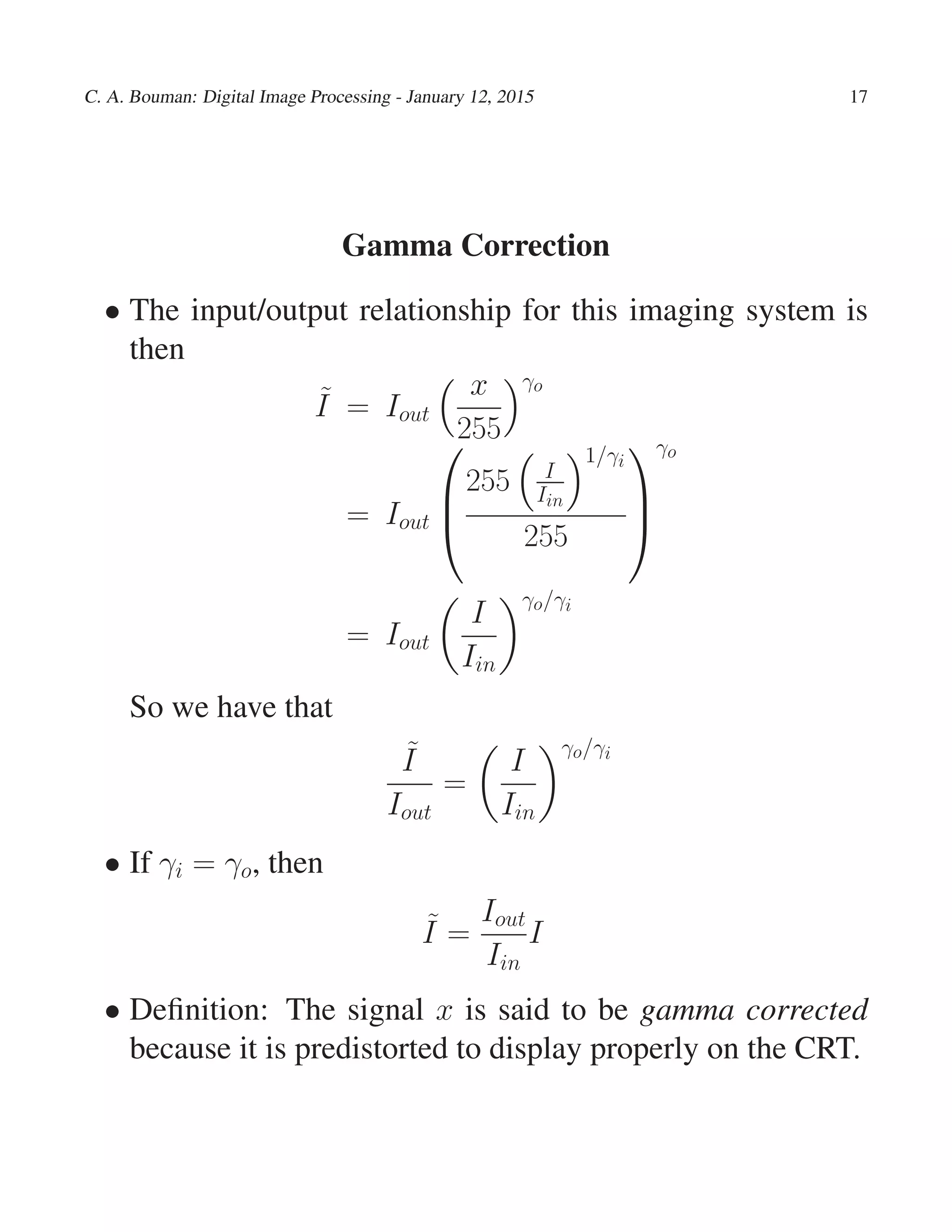
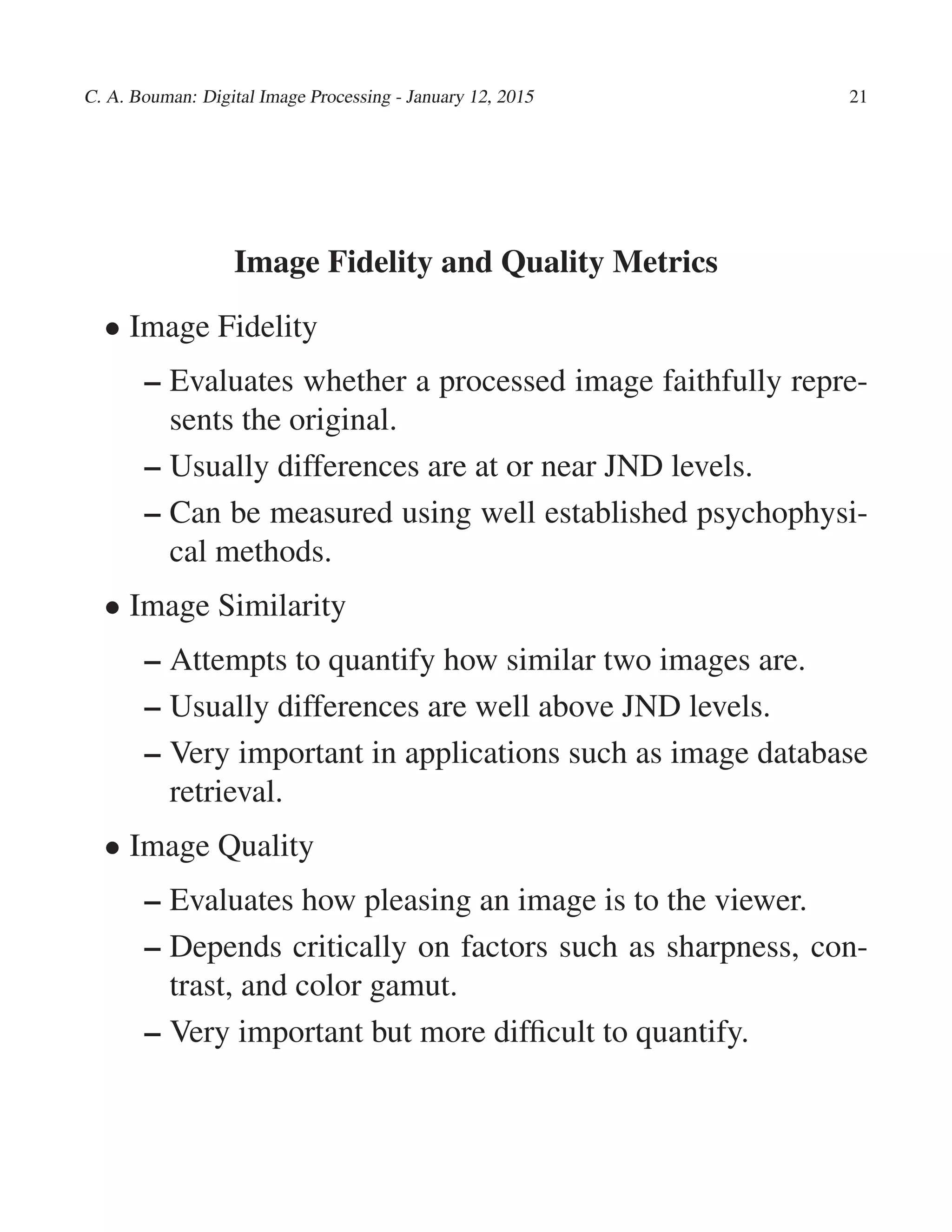
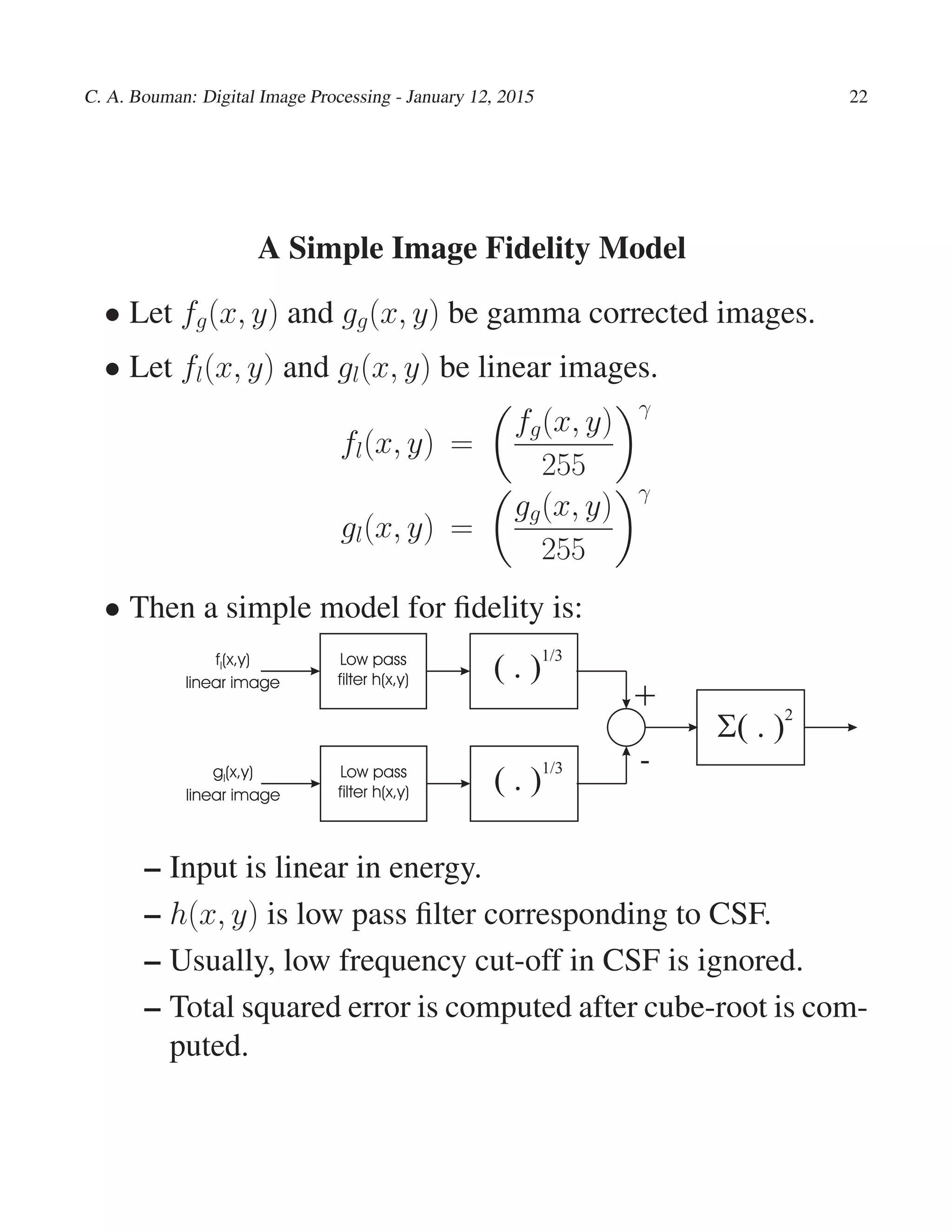
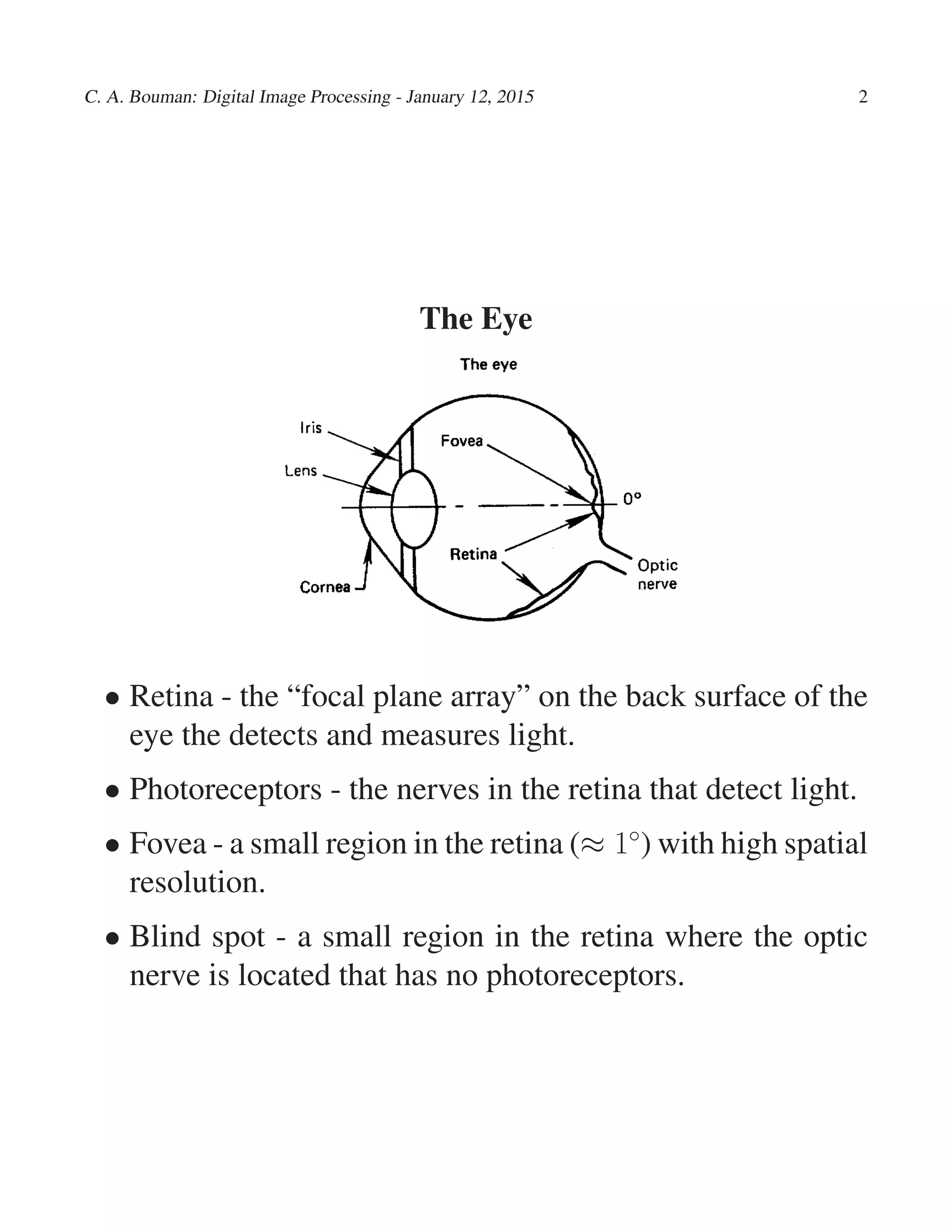
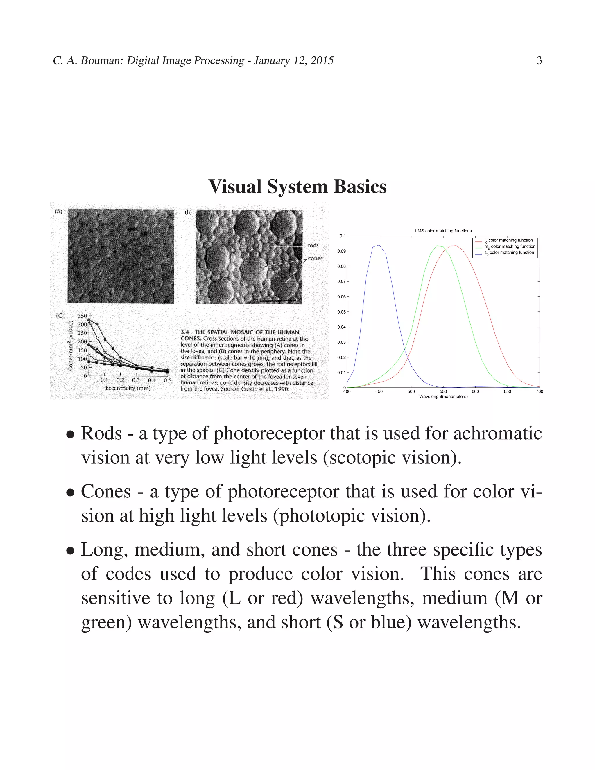
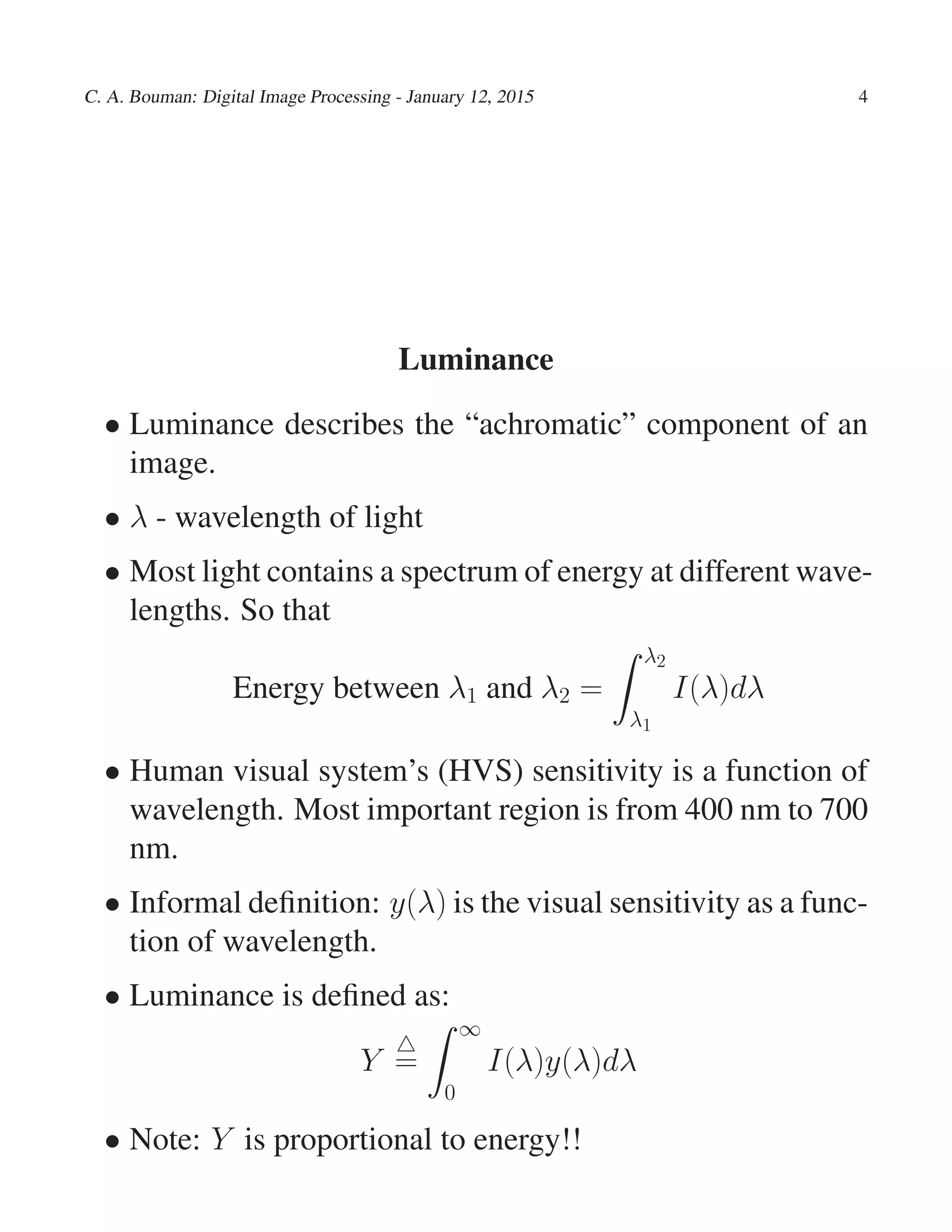
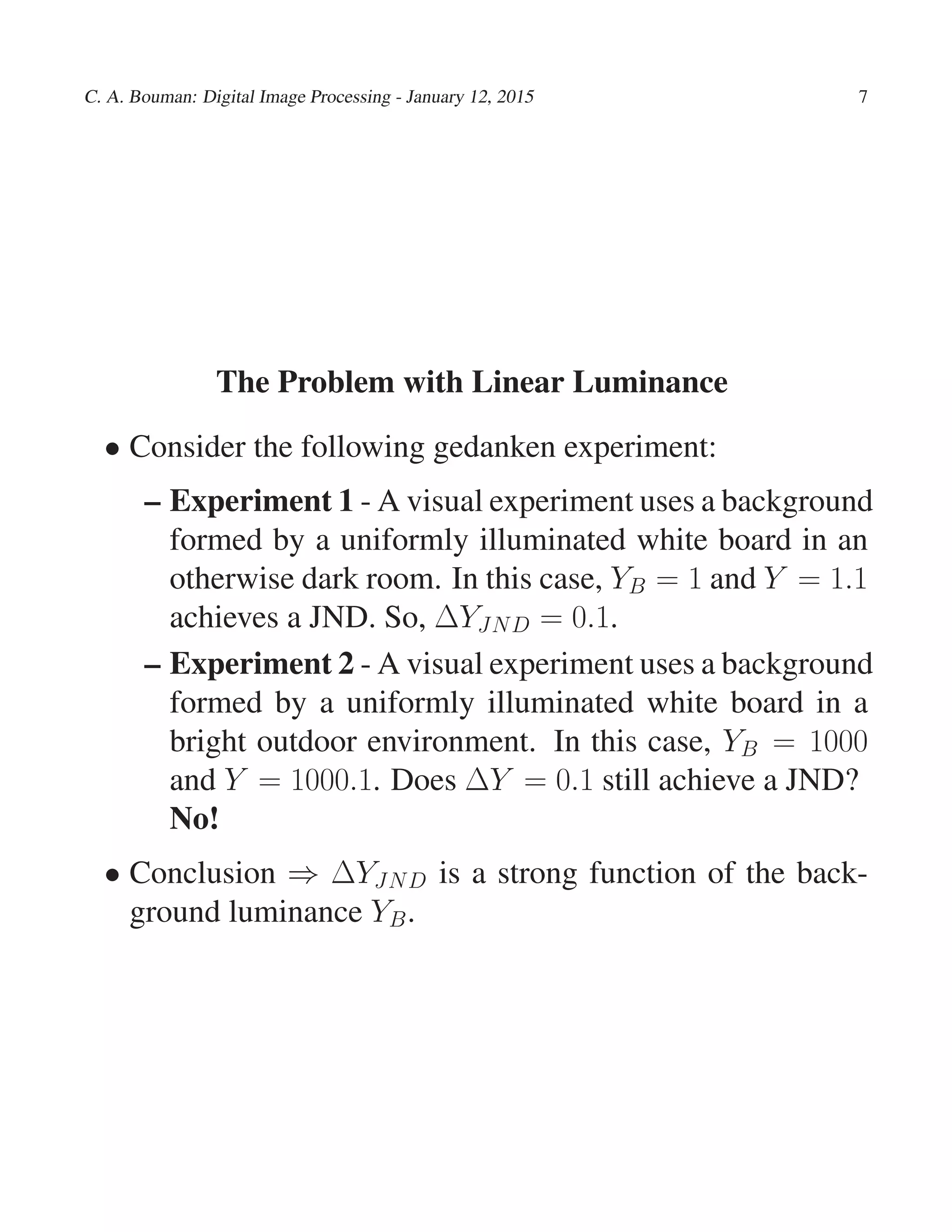
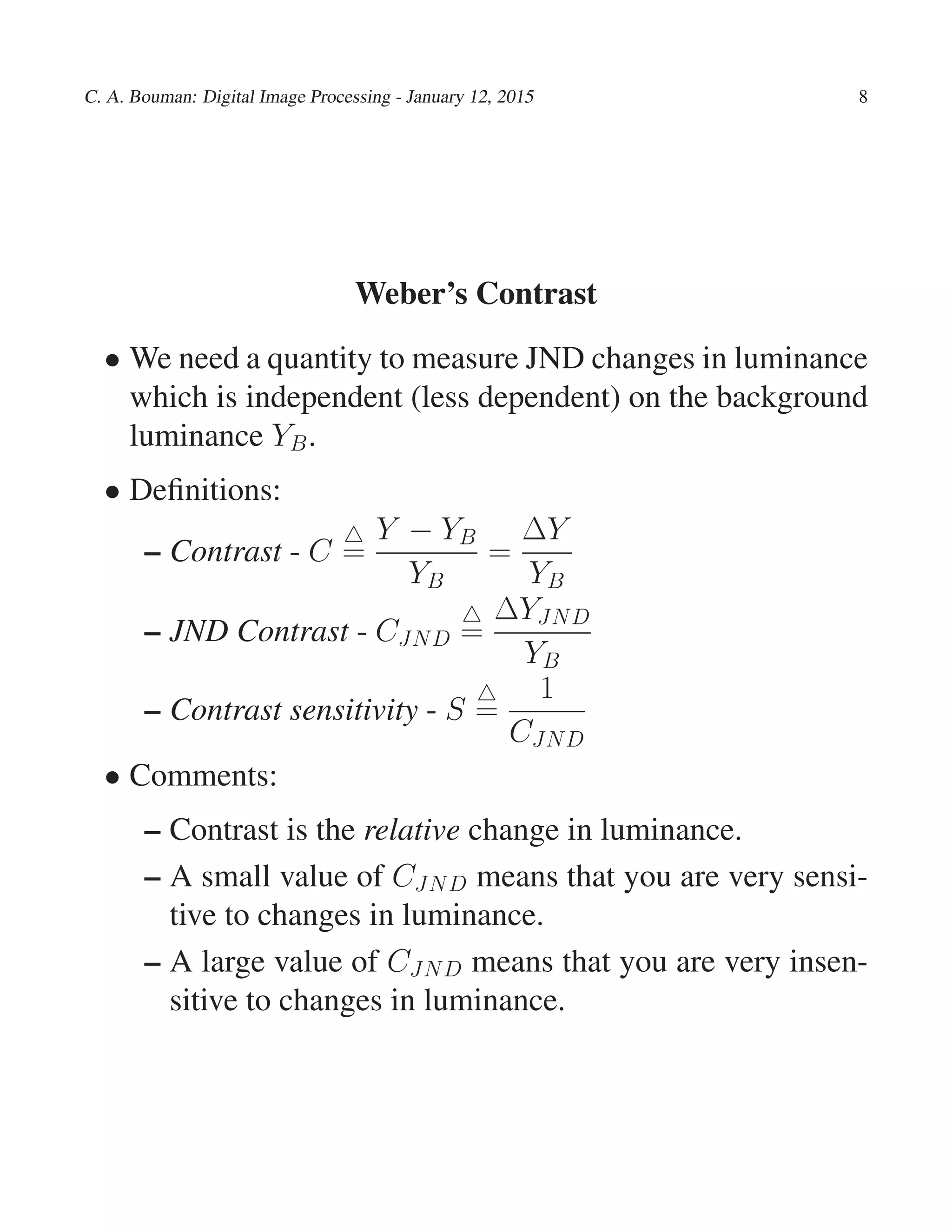
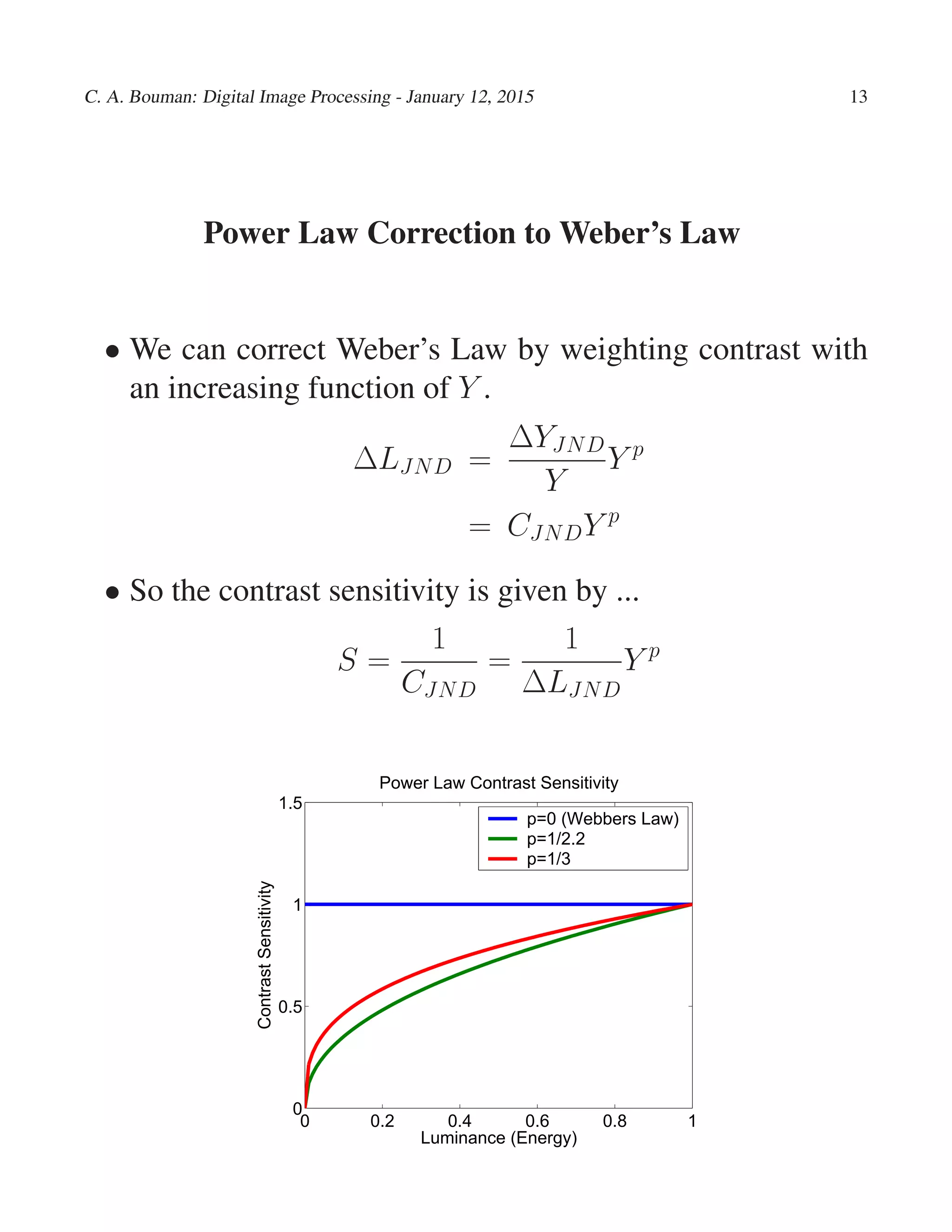
This document discusses how humans perceive visual stimuli and images. It covers topics like the anatomy of the eye, luminance, contrast, color perception, and models of visual sensitivity. Some key points: - The retina detects light and contains photoreceptors like rods and cones that are sensitive to different wavelengths. The fovea provides high spatial resolution. - Luminance describes the achromatic component of an image and is proportional to energy. Contrast is a better measure of visual differences than linear changes in luminance. 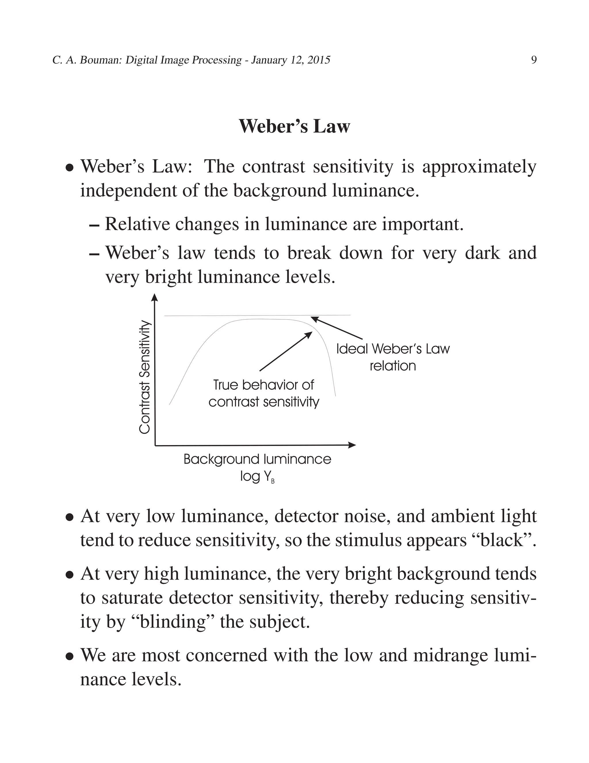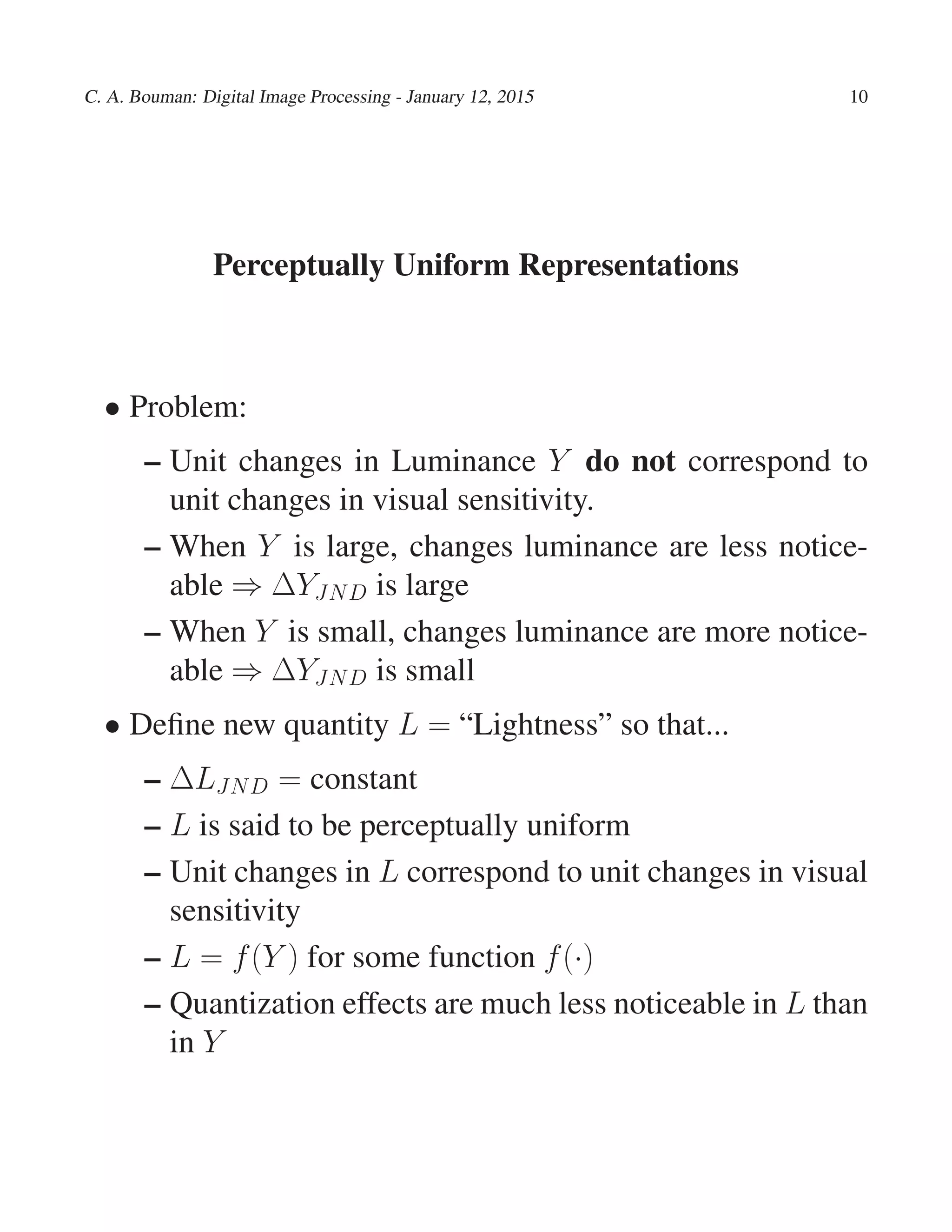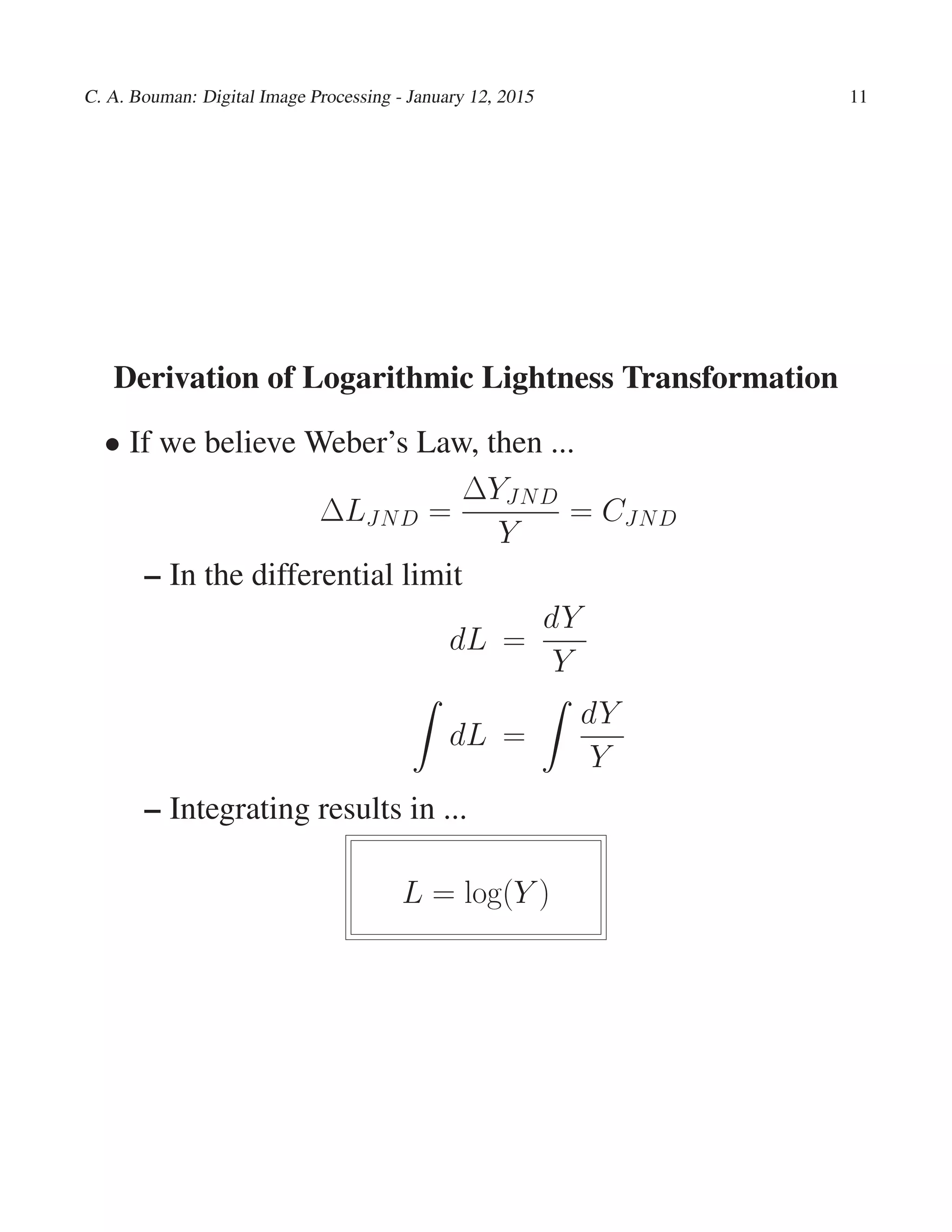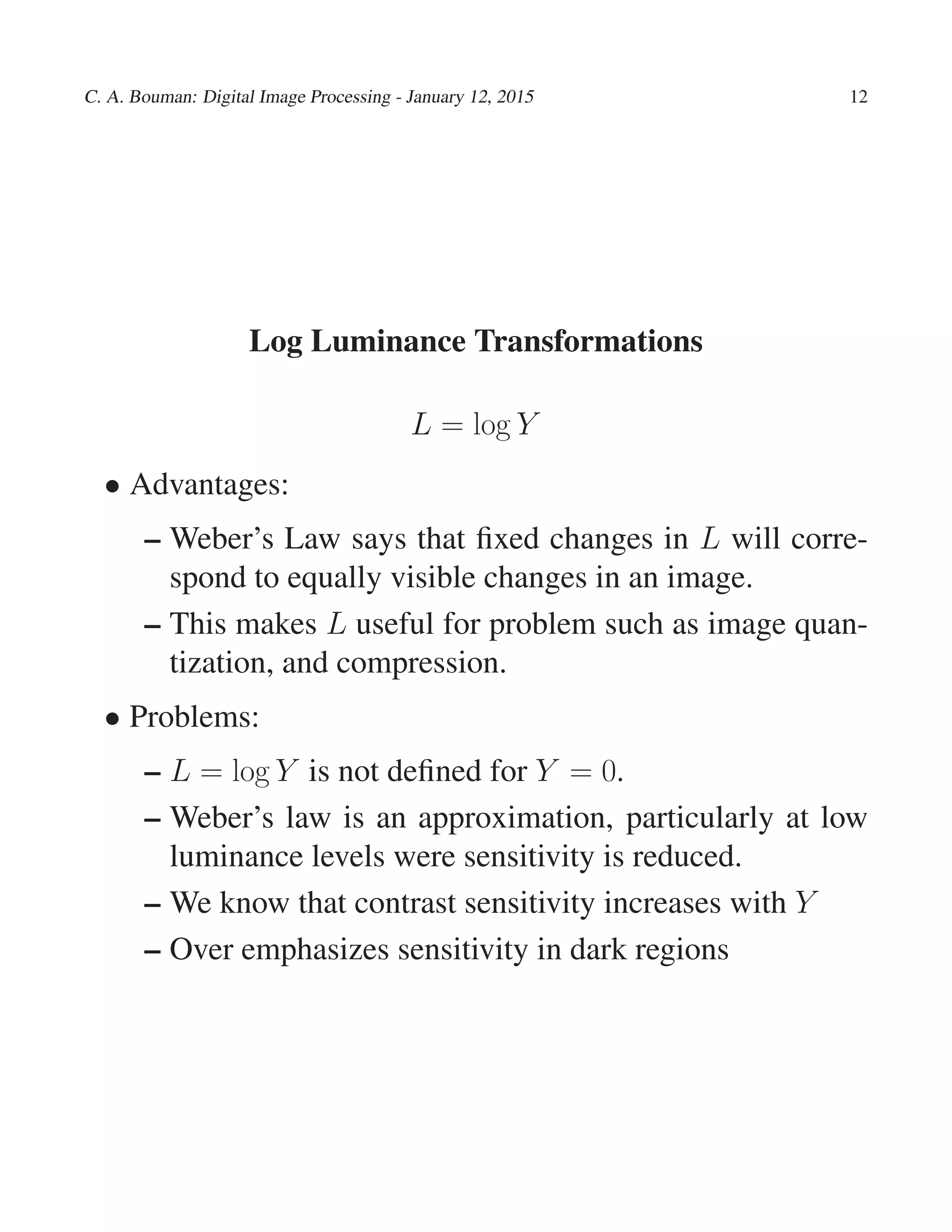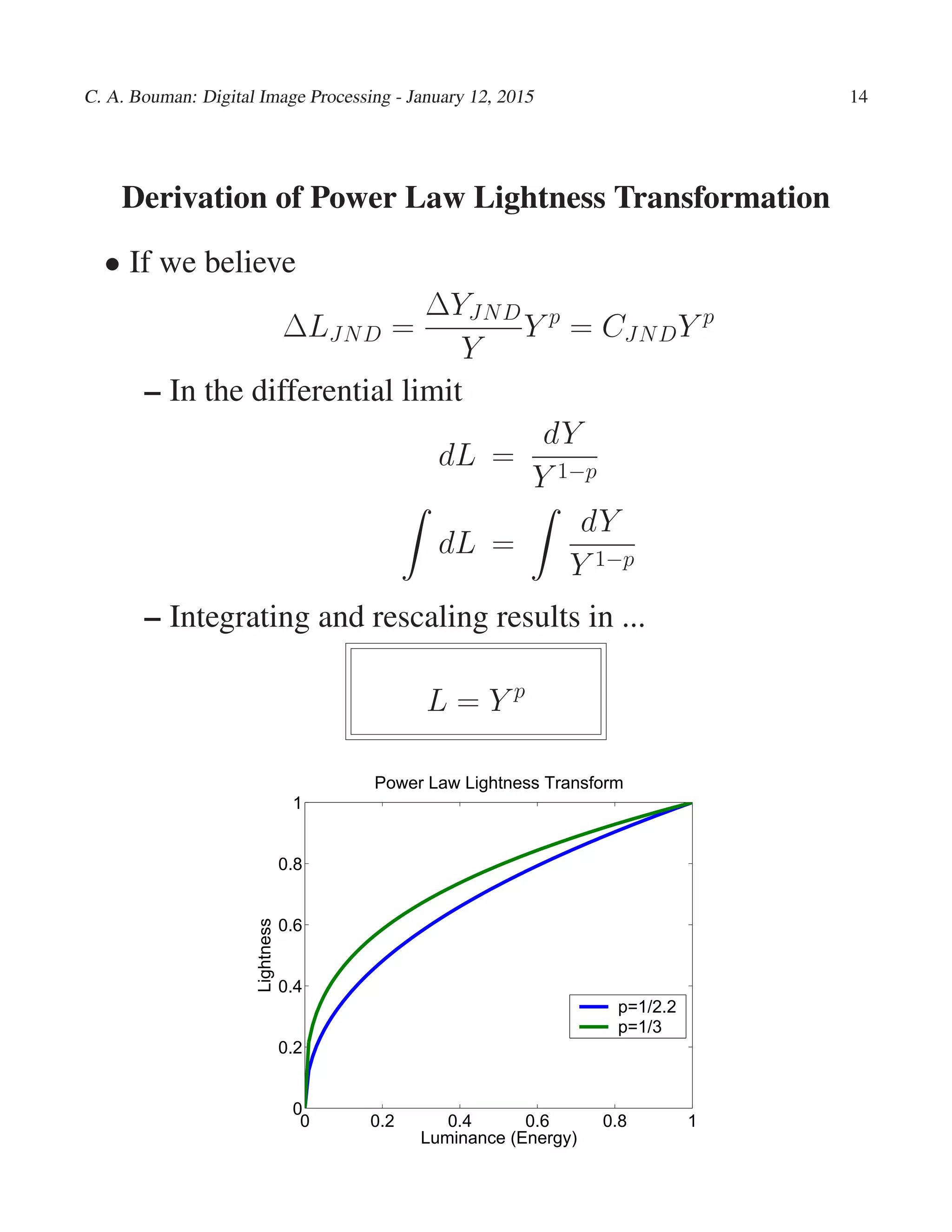- Weber's law and power law transformations model how visual sensitivity depends on background luminance in a perceptually uniform way. 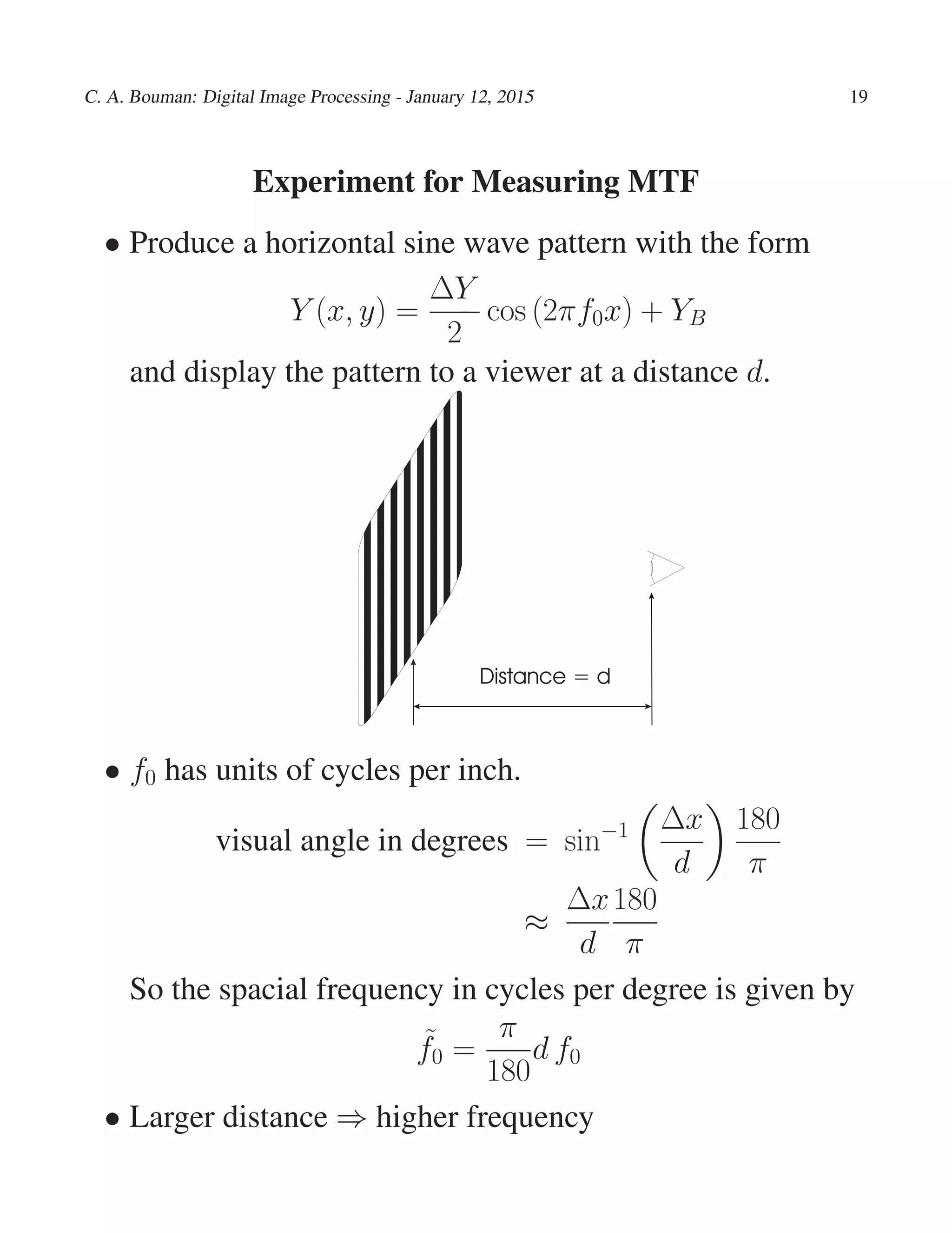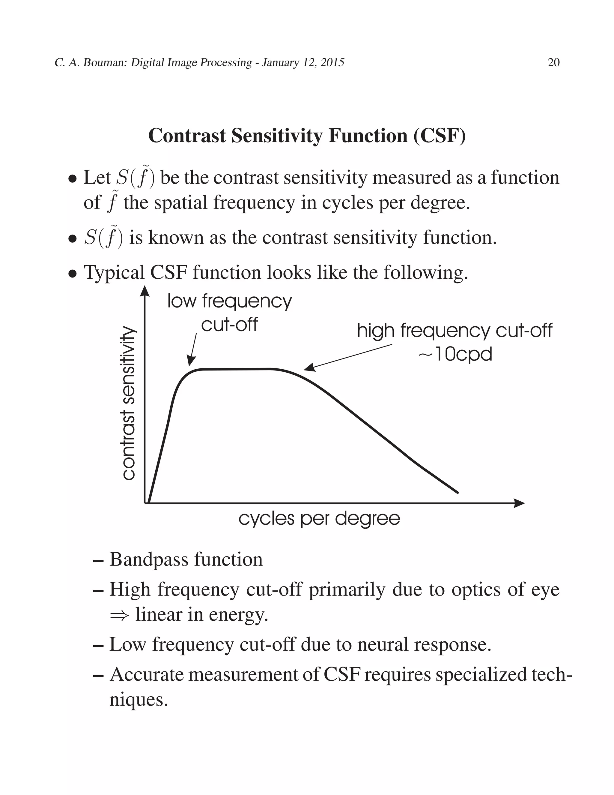- The contrast sensitivity function measures sensitivity to spatial frequencies and

1. C. A. Bouman: Digital Image Processing - January 12, 2015 1
The Visual Perception of Images
• In order to understand “images” you must understand how
humans perceive visual stimulus.
• Objectives:
– Understand contrast and how humans detect changes
in images.
– Understand photometric properties of the physical world.
– Understand the percept of “color”.
– Learn how to use this understanding to design imaging
systems.

2. C. A. Bouman: Digital Image Processing - January 12, 2015 2
The Eye
• Retina - the “focal plane array” on the back surface of the
eye the detects and measures light.
• Photoreceptors - the nerves in the retina that detect light.
• Fovea - a small region in the retina (≈ 1◦
) with high spatial
resolution.
• Blind spot - a small region in the retina where the optic
nerve is located that has no photoreceptors.

3. C. A. Bouman: Digital Image Processing - January 12, 2015 3
Visual System Basics
400 450 500 550 600 650 700
0
0.01
0.02
0.03
0.04
0.05
0.06
0.07
0.08
0.09
0.1
LMS color matching functions
Wavelenght(nanometers)
l0
color matching function
m
0
color matching function
s0
color matching function
• Rods - a type of photoreceptor that is used for achromatic
vision at very low light levels (scotopic vision).
• Cones - a type of photoreceptor that is used for color vi-
sion at high light levels (phototopic vision).
• Long, medium, and short cones - the three specific types
of codes used to produce color vision. This cones are
sensitive to long (L or red) wavelengths, medium (M or
green) wavelengths, and short (S or blue) wavelengths.

4. C. A. Bouman: Digital Image Processing - January 12, 2015 4
Luminance
• Luminance describes the “achromatic” component of an
image.
• λ - wavelength of light
• Most light contains a spectrum of energy at different wave-
lengths. So that
Energy between λ1 and λ2 =
λ2
λ1
I(λ)dλ
• Human visual system’s (HVS) sensitivity is a function of
wavelength. Most important region is from 400 nm to 700
nm.
• Informal definition: y(λ) is the visual sensitivity as a func-
tion of wavelength.
• Luminance is defined as:
Y
△
=
∞
0
I(λ)y(λ)dλ
• Note: Y is proportional to energy!!

5. C. A. Bouman: Digital Image Processing - January 12, 2015 5
400 450 500 550 600 650 700
0
0.01
0.02
0.03
0.04
0.05
0.06
0.07
0.08
0.09
0.1
Typical Relative Luninance Efficiency Function
Wavelenght(nanometers)

6. C. A. Bouman: Digital Image Processing - January 12, 2015 6
A Simple Visual Stimulus
• A single uniform dot of luminance Y (≈ 10◦
) in a large
uniform background of luminance YB.
Background of
luminance YB
Spot of
luminance Y
Question: How much difference is necessary for a “stan-
dard observer” to notice the difference between Y and
YB?
• Definitions:
– The just noticeable difference (JND) is the difference
that allows an observer to detect the center stimulus
50% of the time.
– ∆YJND is the difference in Y and YB required to achieve
a just noticeable difference.

7. C. A. Bouman: Digital Image Processing - January 12, 2015 7
The Problem with Linear Luminance
• Consider the following gedanken experiment:
– Experiment 1 - A visual experiment uses a background
formed by a uniformly illuminated white board in an
otherwise dark room. In this case, YB = 1 and Y = 1.1
achieves a JND. So, ∆YJND = 0.1.
– Experiment 2 - A visual experiment uses a background
formed by a uniformly illuminated white board in a
bright outdoor environment. In this case, YB = 1000
and Y = 1000.1. Does ∆Y = 0.1 still achieve a JND?
No!
• Conclusion ⇒ ∆YJND is a strong function of the back-
ground luminance YB.

8. C. A. Bouman: Digital Image Processing - January 12, 2015 8
Weber’s Contrast
• We need a quantity to measure JND changes in luminance
which is independent (less dependent) on the background
luminance YB.
• Definitions:
– Contrast - C
△
=
Y − YB
YB
=
∆Y
YB
– JND Contrast - CJND
△
=
∆YJND
YB
– Contrast sensitivity - S
△
=
1
CJND
• Comments:
– Contrast is the relative change in luminance.
– A small value of CJND means that you are very sensi-
tive to changes in luminance.
– A large value of CJND means that you are very insen-
sitive to changes in luminance.

9. C. A. Bouman: Digital Image Processing - January 12, 2015 9
Weber’s Law
• Weber’s Law: The contrast sensitivity is approximately
independent of the background luminance.
– Relative changes in luminance are important.
– Weber’s law tends to break down for very dark and
very bright luminance levels.
Ideal Weber’s Law
relation
True behavior of
contrast sensitivity
Background luminance
log YB
ContrastSensitivity
• At very low luminance, detector noise, and ambient light
tend to reduce sensitivity, so the stimulus appears “black”.
• At very high luminance, the very bright background tends
to saturate detector sensitivity, thereby reducing sensitiv-
ity by “blinding” the subject.
• We are most concerned with the low and midrange lumi-
nance levels.

10. C. A. Bouman: Digital Image Processing - January 12, 2015 10
Perceptually Uniform Representations
• Problem:
– Unit changes in Luminance Y do not correspond to
unit changes in visual sensitivity.
– When Y is large, changes luminance are less notice-
able ⇒ ∆YJND is large
– When Y is small, changes luminance are more notice-
able ⇒ ∆YJND is small
• Define new quantity L = “Lightness” so that...
– ∆LJND = constant
– L is said to be perceptually uniform
– Unit changes in L correspond to unit changes in visual
sensitivity
– L = f(Y ) for some function f(·)
– Quantization effects are much less noticeable in L than
in Y

11. C. A. Bouman: Digital Image Processing - January 12, 2015 11
Derivation of Logarithmic Lightness Transformation
• If we believe Weber’s Law, then ...
∆LJND =
∆YJND
Y
= CJND
– In the differential limit
dL =
dY
Y
dL =
dY
Y
– Integrating results in ...
L = log(Y )

12. C. A. Bouman: Digital Image Processing - January 12, 2015 12
Log Luminance Transformations
L = log Y
• Advantages:
– Weber’s Law says that fixed changes in L will corre-
spond to equally visible changes in an image.
– This makes L useful for problem such as image quan-
tization, and compression.
• Problems:
– L = log Y is not defined for Y = 0.
– Weber’s law is an approximation, particularly at low
luminance levels were sensitivity is reduced.
– We know that contrast sensitivity increases with Y
– Over emphasizes sensitivity in dark regions

13. C. A. Bouman: Digital Image Processing - January 12, 2015 13
Power Law Correction to Weber’s Law
• We can correct Weber’s Law by weighting contrast with
an increasing function of Y .
∆LJND =
∆YJND
Y
Y p
= CJNDY p
• So the contrast sensitivity is given by ...
S =
1
CJND
=
1
∆LJND
Y p
0 0.2 0.4 0.6 0.8 1
0
0.5
1
1.5
Power Law Contrast Sensitivity
ContrastSensitivity
Luminance (Energy)
p=0 (Webbers Law)
p=1/2.2
p=1/3

14. C. A. Bouman: Digital Image Processing - January 12, 2015 14
Derivation of Power Law Lightness Transformation
• If we believe
∆LJND =
∆YJND
Y
Y p
= CJNDY p
– In the differential limit
dL =
dY
Y 1−p
dL =
dY
Y 1−p
– Integrating and rescaling results in ...
L = Y p
0 0.2 0.4 0.6 0.8 1
0
0.2
0.4
0.6
0.8
1
Luminance (Energy)
Lightness
Power Law Lightness Transform
p=1/2.2
p=1/3

15. C. A. Bouman: Digital Image Processing - January 12, 2015 15
Power Law Luminance Transformations
L = Y p
• L is well defined for Y = 0.
• L models the reduced sensitivity at low luminance levels.
• p = 1/3 is known to fit empirical data well.
• p = 1/2.2 is more robust and is widely used in applica-
tions.
• We will see that p = 1
γ where γ is the parameter used in
“gamma correction.”
• Typical values of p:
– NTSC video p = 1/2.2
– sRGB color standard p = 1/2.2
– Standard PC and Unix displays p = 1/2.2
– MacIntosh computers p = 1/1.8
– L∗
a∗
b∗
visually uniform color space p = 1/3

16. C. A. Bouman: Digital Image Processing - January 12, 2015 16
Input and Output Nonlinearities in Imaging Systems
I
Incoming light intensity x
Digitized signal
I
Displayed light intensity
A/D CRT
Display
device
Vidicon tube
used for
image capture
Digital Image
transmision
or storage
D/A
~
• x(m, n) generally takes values from 0 to 255
• Videcon tubes are (were) nonlinear with input/output re-
lationship.
x = 255
I
Iin
1/γi
where Iin is the maximum input, and γi is a parameter of
the input device.
• The cathode ray tube (CRT) has the inverse input/output
relationship.
˜I = Iout
x
255
γo
where Iout is the maximum output and γo is a parameter
of the output device.

17. C. A. Bouman: Digital Image Processing - January 12, 2015 17
Gamma Correction
• The input/output relationship for this imaging system is
then
˜I = Iout
x
255
γo
= Iout



255 I
Iin
1/γi
255



γo
= Iout
I
Iin
γo/γi
So we have that
˜I
Iout
=
I
Iin
γo/γi
• If γi = γo, then
˜I =
Iout
Iin
I
• Definition: The signal x is said to be gamma corrected
because it is predistorted to display properly on the CRT.

18. C. A. Bouman: Digital Image Processing - January 12, 2015 18
Visual MTF
• How do we quantify the spacial frequency response of the
visual system?
• Answer: Measure the contrast sensitivity as a function of
spatial frequency.

19. C. A. Bouman: Digital Image Processing - January 12, 2015 19
Experiment for Measuring MTF
• Produce a horizontal sine wave pattern with the form
Y (x, y) =
∆Y
2
cos (2πf0x) + YB
and display the pattern to a viewer at a distance d.
Distance = d
• f0 has units of cycles per inch.
visual angle in degrees = sin−1 ∆x
d
180
π
≈
∆x
d
180
π
So the spacial frequency in cycles per degree is given by
˜f0 =
π
180
d f0
• Larger distance ⇒ higher frequency

20. C. A. Bouman: Digital Image Processing - January 12, 2015 20
Contrast Sensitivity Function (CSF)
• Let S( ˜f) be the contrast sensitivity measured as a function
of ˜f the spatial frequency in cycles per degree.
• S( ˜f) is known as the contrast sensitivity function.
• Typical CSF function looks like the following.
contrastsensitivity
cycles per degree
high frequency cut-off
~10cpd
low frequency
cut-off
– Bandpass function
– High frequency cut-off primarily due to optics of eye
⇒ linear in energy.
– Low frequency cut-off due to neural response.
– Accurate measurement of CSF requires specialized tech-
niques.

21. C. A. Bouman: Digital Image Processing - January 12, 2015 21
Image Fidelity and Quality Metrics
• Image Fidelity
– Evaluates whether a processed image faithfully repre-
sents the original.
– Usually differences are at or near JND levels.
– Can be measured using well established psychophysi-
cal methods.
• Image Similarity
– Attempts to quantify how similar two images are.
– Usually differences are well above JND levels.
– Very important in applications such as image database
retrieval.
• Image Quality
– Evaluates how pleasing an image is to the viewer.
– Depends critically on factors such as sharpness, con-
trast, and color gamut.
– Very important but more difficult to quantify.

22. C. A. Bouman: Digital Image Processing - January 12, 2015 22
A Simple Image Fidelity Model
• Let fg(x, y) and gg(x, y) be gamma corrected images.
• Let fl(x, y) and gl(x, y) be linear images.
fl(x, y) =
fg(x, y)
255
γ
gl(x, y) =
gg(x, y)
255
γ
• Then a simple model for fidelity is:
f(x,y)
linear image
l
+
-
Low pass
filter h(x,y) ( . )
1/3
S( . )2
gl(x,y)
linear image
Low pass
filter h(x,y) ( . )1/3
– Input is linear in energy.
– h(x, y) is low pass filter corresponding to CSF.
– Usually, low frequency cut-off in CSF is ignored.
– Total squared error is computed after cube-root is com-
puted.