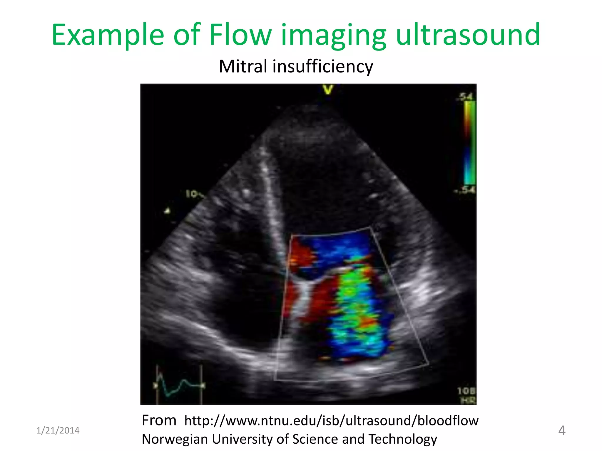
The document discusses a flow imaging cardiac ultrasound system developed by Dr. Larry Miller, detailing its technology, architecture, and operational parameters. The goal of the system is to produce real-time grayscale anatomical images of the heart superimposed with blood flow velocities indicated in color. The document also outlines electronic and signal processing techniques used to enhance the imaging and detection of blood flow during cardiac examinations.

1. Flow Imaging Cardiac
Ultrasound system
by Larry Miller PhD
www.linkedin.com/in/lrmiller
miller@elect-design.com
US Patent 4,612,937
Ultrasound Diagnostic Apparatus,
Inventor: Lawrence (Larry) R Miller
11/21/2014

2. Cardiac ultrasound technology existing
at start of project
• Anatomical imaging ultrasound
– Manually aimed and rotated for desired fan
placement. Produces 2D fan image
– Observe heart wall motion, valve leaflet motion, etc.
• Display: 2D fan-shaped grayscale reflectivity image: Heart
structures are reflective, blood shows minimally visible
reflectivity.
• Doppler probe
– Manually aimed in desired direction
– Shows blood velocity as a function of depth (distance
from probe along the 1-dimensional beam)
• Display: strip chart similar to a sonogram V=depth, H=time
21/21/2014

3. Project goal:
Flow-imaging cardiac ultrasound
Requirements
– Display real-time anatomical image of heart and
related structures as grayscale
– Superimpose image of blood flowing towards the
probe in red and away from the probe in blue
51/21/2014

4. Example of Flow imaging ultrasound
Mitral insufficiency
From http://www.ntnu.edu/isb/ultrasound/bloodflow
Norwegian University of Science and Technology
41/21/2014

5. Flow imager pulse sequence
• Ultrasound frequency f0
– 3.5 MHz. This is typical for cardiac ultrasound as it
provides adequate penetration depth. λ = 0.43 mm.
• Pulse sequence
– N pulses in a given direction them move to the next
direction
– Frequency resolution increases with increasing N. N=5
chosen for first prototype
• Pulse repetition rate
– A typical cardiac image will be 10 cm deep
– Speed of sound in tissue and water c = 150,000 cm./sec.
– Pulse rate thus Fpulse = 7500 pulses per second.
51/21/2014

6. Flow imager architecture
• Single element oscillating probe vs phased array
probe
– Acquiring Doppler signal requires multiple pulses in
the same direction before moving to the next
direction
– Oscillating probe cannot perform move and stop,
move and stop, … thus phased array probe needed
• Added advantage: phased array probe allows dynamic
receive focus, providing greater effective depth of focus
61/21/2014

7. Doppler velocity detection parameters
• Max unambiguous blood velocity ±vmax
– Nyquist: max unambiguous Fd is Fpulse / 2 which is 3750 Hz
– Backscatter Doppler frequency Fd = 2 f0 v / c where v is
blood velocity. v = Fd c / (2 f0 )
– Practical max. for 5 pulse sequence is 80% of Nyquist
– vmax = 0.8 x 3750 x 150,000 / (2 x 3.5 x 106 ) = 64 cm. / sec.
• Interleaving
– An interleaved by m pulse sequence will have vmax = (64 /
m) cm./sec. This mode is used for observing flows with
lower peak velocities.
71/21/2014

8. Flow imager fan
• Fan width: 90 degrees
• Probe elements:
– linear array of 32 elements
– Lead zirconate titanate (PZT) (ATL Technologies)
– dielectric constant 700
– Longitudinal resonance thru thickness: 3.5 MHz
– Backed by carbon loaded silicone:
reduces Q of longitudinal resonance to 3
• Probe Dimensions
– 15 mm wide by 10 mm high
81/21/2014

9. Array patterns
Single element response
91/21/2014

10. Array patterns
• Array response for four steering angles
Infinite focus case 101/21/2014

11. Blood velocity estimator
• Requirements
– Should not respond to low velocities.
– Should use a minimal number of pulse samples in order to
achieve high frame rate
• Vest(beam_direction,depth_bin) =
abs ( 1
5
𝑐[𝑖] ∗ 𝑑[𝑖])2 – abs ( 1
5
𝑐𝑜𝑛𝑗(𝑐 𝑖 ) ∗ 𝑑[𝑖])2
– c[i] are 5 fixed coefficients: 1-2i, -4+4i, 6, -4-4i, 1+2i
– d[i] are 5 consecutive data points for 5 consecutive pulses along
the given beam direction in the given depth bin
111/21/2014

12. Blood velocity estimator
• Doppler frequency estimator response function
Nyquist band
Relation between velocity and Doppler frequency: v = Fd c / (2 f0 )
121/21/2014

13. Electronic block diagram
32 piezoelectric
element ultrasound
probe
32 element
driver/receiver
boards
Receive signal
combiner
A to D
converter
Digital
controller
Log amplifier
& detector
Polar to
rectangular
scan
converter
2 x D to A
converter
Color
NTSC
formatter
Display
Digital
Doppler
processor
cable
Blood
veloc.
Anatom.
image
…
131/21/2014

14. Element Driver/Receive board
Probe
element
Fine delay
line
0.05 μs/tap
Coarse
delay line
0.5 μs/tap
mux mux
Static
RAM
Memory download and control from
backplane
Combined
analog receive
signal
(drive to
backplane analog
bus)
14
Outputs change during
receive interval to
implement dynamic focus
Matching
network &
Preamplifier
agc1
agc2 agc3 agc4
3 subsequent
gain-controlled
amplifier stages
Pulse
generator
1/21/2014

15. Doppler processor electronics
Doppler processor detail
I and Q
demodulator
and digitizer
Combined
analog
receive signal
3 MHz
transmit
oscillator
output
Digital logic
Blood velocity signal
15
From US Patent 4,612,937
1/21/2014

16. Matching network and preamplifier
(simplified – parasitic snubbing resistors omitted)
V supply
Probe
element
equivalent
circuit +V
bias
Cascode
stage
Lp
Cp
Rp
Lt
Cf (4 x parasitic cap. G to S) = 16 pF
Lt = 14.6 uH Cp = 10 pF Lp = 220 uH
Rp = 1.6 kOhm Cc = 134 pF
G
S
Voltage source
proportional to
ultrasound signal
G
S S
G
S
G
Preamp
output to
next stage
Zload
4 x
2N4416
JFET
AGC in
Cc
16
-I bias
+I bias
Pulse in1/21/2014

17. Preamplifier Noise Figure
• Noise Figure at 3.5 MHz
– NF = 20 log (Vt / Vs)
• A measure of noise added by the preamplifier
• Vt = total noise voltage per 𝐻𝑧 at preamp output
• Vs = noise voltage contributed by source resistance Rp per 𝐻𝑧 at preamp output
– Vs = G 4 kTRp per 𝐻𝑧 = 4.4 nV per 𝐻𝑧
• G = preamplifier gain E/e
– Vt = 𝑉 𝑠
2 + 𝑉𝑛2
• 𝑉 𝑛 = 3 nanovolts per 𝐻𝑧
» Each JFET has 6 nV per 𝐻𝑧 noise, so 4 averaged provides 3 nV per
– = 5.32 / 4.4 = 1.21
– NF = 1.65 dB
171/21/2014

18. Probe and matching network
frequency response
Frequency (MHz)
Relative
response
amplitude
Half power band: 3.0 MHz to 3.9 MHz
181/21/2014

19. Probe and preamp input network
impulse response
Envelope full width half maximum = 0.88 microseconds
Corresponds to 0.66 mm depth range.
Thus depth resolution is 0.66 mm
191/21/2014

20. Automatic Gain Control (AGC)
• Four successive AGC amplifier stages
starting with preamp
– Chart shows control voltage applied to each of these 4
stages, and the total AGC achieved
– AGC in voltage
is linearly related
to 10gain_in_dB/20
– AGC in voltages ramps are
Generated from table
Driving DAC
201/21/2014

21. Log amplifier
simplified schematic
3 of 6 stages shown
21
-supply -supply
Output
-supply
+supply
Input
-supply
Current
mirror
Detector
stages
HF limiting
amplifier
stages
(Bandpass
filtering not
shown)
-bias
R R RR/6
Detector
zero
reference
1/21/2014

22. Log amplifier stage transfer functions
22
• HF limiting amplifier stage
transfer function
• (exp (Ein/2) - exp(-Ein/2))/(exp (Ein/2) +
exp(-Ein/2))
• E0 = kT/q ≈ 27 mV.
• Ein =
stage input voltage / E0
• Stage output voltage =
Gain * Eout * E0
• Gain = 10 dB
• Detector stage transfer
function
• Detector: Eout = log(1 + exp (Ein))
• Ein = detector input voltage / E0
• Detector output voltage = Eout * E0
1/21/2014

23. Log Amplifier transfer function
from model
23
• Gain 20 dB per
differential
amplifier stage
• Gain 10 dB per
differential
amplifier stage
Input signal level in dB
Output signal
level
linear scale
Output signal
level
linear scale
• This gain per stage
was used for
prototype
1/21/2014

24. Dynamic apodization
• Contributions from elements at each end
reduced for first 1 cm.
– Reduces sensitivity to reflections from adjacent ribs
– Method: agc for outer elements reduced over first 1 cm.
241/21/2014

25. Scan Converter
10 cm. depth mode: 0.39 mm. per raster line
25
Raster
lines
1
2
256
Raster lines 1
to 256
Scan convert
on write
Raster lines 17
to 256
Scan convert on
read
128 beam directions
Raster scanout: 2048 pixels in 40 μsec 50 MHz output pixel clock1/21/2014

26. Scan Converter
10 cm. depth mode: 0.39 mm. per raster line
26
Raster
lines
1
2
256
Raster lines 1
to 256
Scan convert
on write
Raster lines 17
to 256
Scan convert on
read
128 beam directions
Raster scanout: 2048 pixels in 40 μsec 50 MHz output pixel clock1/21/2014

27. Clinical tests of prototypes
• Approvals and tests
– Preapproved by review board at all medical facilities
where tested as investigational device exemption
– Substantially equivalent to Toshiba diagnostic ultrasound
device. Same power levels, repetition rate, probe area,
and general function.
– Tested by cardiologists at ten hospitals
• Results
– Image rated very good and flow imaging worked well on
most patients.
– No interference artifact (because of good isolation of
sensitive electronics from digital electronics)
271/21/2014

28. Appendix
• FDA output limits for diagnostic ultrasound
– A spatial-peak temporal-average intensity (ISPTA) less than 720 mW/cm2.
– The acoustic output depends on the output power, pulse repetition
frequency, and scanner operating mode (eg, B-mode, M-mode, pulsed, or
color or power Doppler imaging).4,9
– J Ultrasound Med 2009; 28:139–150 141
• Power output of our prototype
– Pulse width: 0.8 microseconds. Min rep period: 133 μsec
– Pulse voltage: 10 volts. Minimum probe impedance: 1600 ohms.
– Max instantaneous power generated: 32 x 102/1600 = 2.0 watts
– Max temporal average power (at spatial peak) 2.0 x 0.8/133 = 12 mW
– Probe active area: 1.6 cm2
– Max spatial peak temporal average power per cm < 7.6 mW
• Probe carbon-loaded silicone backing absorbs some of the energy
281/21/2014