The document discusses association rule mining, a key data mining technique aimed at discovering relationships between items in transactional data. It emphasizes the importance of support and confidence in determining frequent itemsets and generating association rules, utilizing algorithms such as apriori for efficient detection. The document also covers various methods for rule discovery, such as problem decomposition, frequent and maximal frequent sets, and introduces alternative algorithms like the partition and pincer-search algorithms.

1. ASSOCIATION RULE
REFERENCE: DATA MINING TECHNIQUES BY ARUN K. PUJARI
MRS.SOWMYA JYOTHI
SDMCBM
MANGALORE

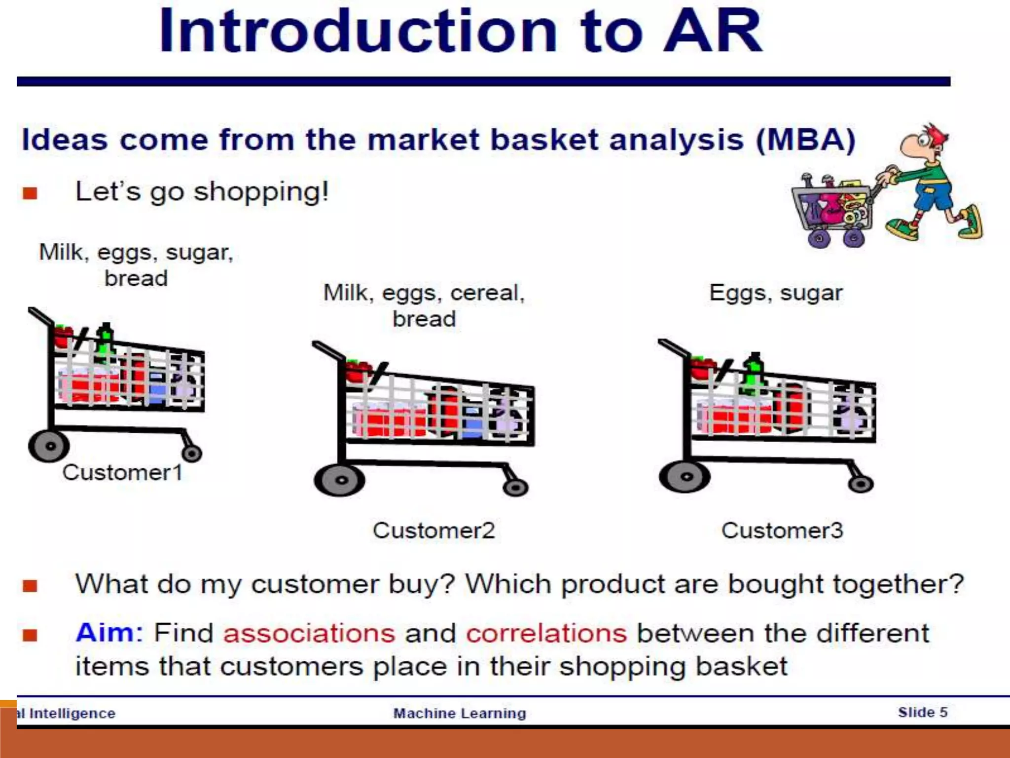
2. INTRODUCTION
Association is to find the association/relation between the items in
the data.
Among the areas of data mining, the problem of deriving
associations from data has received a great deal of attention.
The problem was formulated by Agrawal et al in 1993 and is often
referred to as market basket problem.
In this problem, we are given a set of items and large no. of
transactions [transactions are the subset of these items] which are
subsets(baskets) of these items.
Task is to find the relationships between the various items within
these baskets.

4. There are numerous applications of data mining which
fit into this framework.
The classic example, from which the problem gets its
name, is the supermarket.
In this context, the problem is to analyse customers
buying habits by finding associations between the
different items that customers place in their shopping
baskets.
The discovery of such association rules can help the
retailer develop marketing strategies, by gaining
insight into matters like “which items are most
frequently purchased by customers”. It also helps in
inventory management, sale promotion strategies etc.

5. It is widely accepted that the discovery of association rules
is solely dependent on the discovery of frequent sets.
Thus, a majority of the algorithms are concerned with
efficiently determining the set of frequent itemsets in a
given set of the transaction database. The problem is
essentially to compute the frequency of occurences of
each itemset in the database. Since the total number of
itemsets is exponential in terms of the number of items, it is
not possible to count the frequencies of these sets by
reading the database in just one pass. The number of
counters are too many to be maintained in a single pass. As
a result, using multiple passes to generate all the frequent
itemsets is unavoidable. Thus, different algorithms for the
discovery of association rules aim at reducing the number
of passes by generating candidate sets, which are likely to
be frequent sets.

6. The other problems are
One can ask whether it is possible to find
association rules incrementally. The idea is to avoid
computing the frequent sets afresh for the
incremented set of data. The concept of border sets
become very important in this context.
The discovery of frequent itemsets with item
constraints is one such important related problem.
We shall study the important methods of discovering
association rules in a large database.

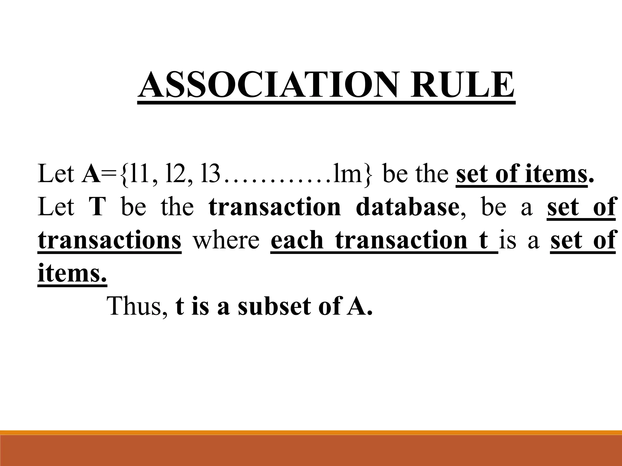
7. ASSOCIATION RULE
Let A={l1, l2, l3…………lm} be the set of items.
Let T be the transaction database, be a set of
transactions where each transaction t is a set of
items.
Thus, t is a subset of A.

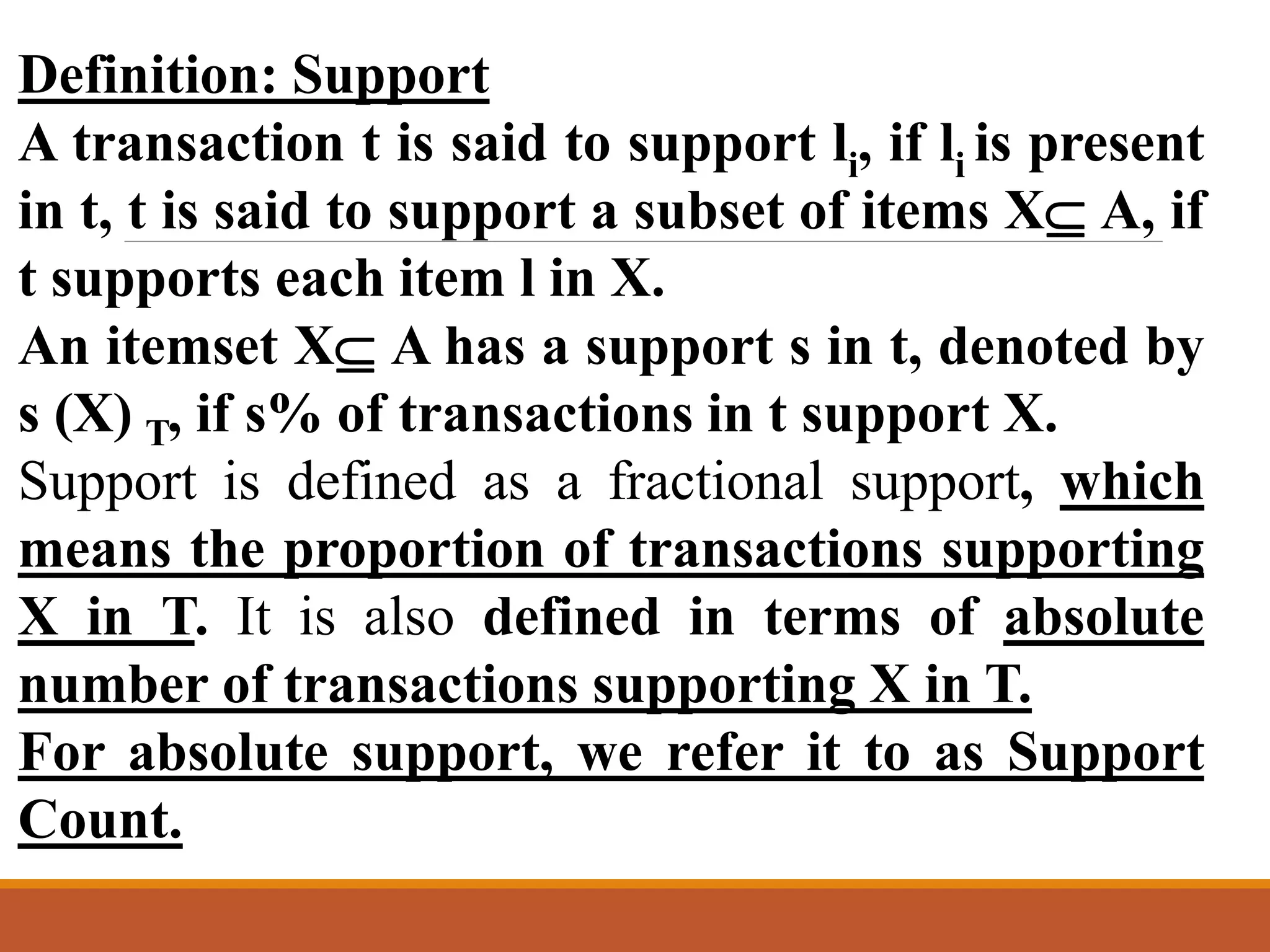
8. Definition: Support
A transaction t is said to support li, if li is present
in t, t is said to support a subset of items X A, if
t supports each item l in X.
An itemset X A has a support s in t, denoted by
s (X) T, if s% of transactions in t support X.
Support is defined as a fractional support, which
means the proportion of transactions supporting
X in T. It is also defined in terms of absolute
number of transactions supporting X in T.
For absolute support, we refer it to as Support
Count.

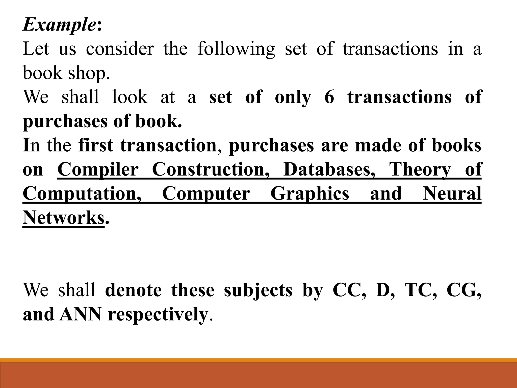
9. Example:
Let us consider the following set of transactions in a
book shop.
We shall look at a set of only 6 transactions of
purchases of book.
In the first transaction, purchases are made of books
on Compiler Construction, Databases, Theory of
Computation, Computer Graphics and Neural
Networks.
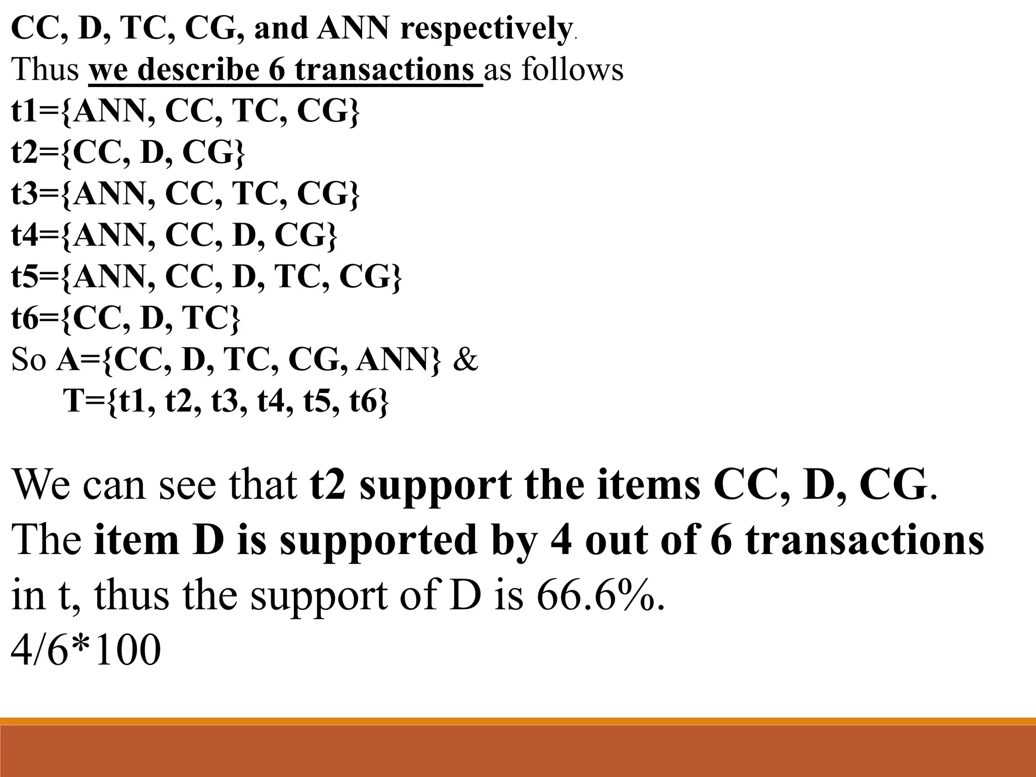
We shall denote these subjects by CC, D, TC, CG,
and ANN respectively.

10. CC, D, TC, CG, and ANN respectively.
Thus we describe 6 transactions as follows
t1={ANN, CC, TC, CG}
t2={CC, D, CG}
t3={ANN, CC, TC, CG}
t4={ANN, CC, D, CG}
t5={ANN, CC, D, TC, CG}
t6={CC, D, TC}
So A={CC, D, TC, CG, ANN} &
T={t1, t2, t3, t4, t5, t6}
We can see that t2 support the items CC, D, CG.
The item D is supported by 4 out of 6 transactions
in t, thus the support of D is 66.6%.
4/6*100

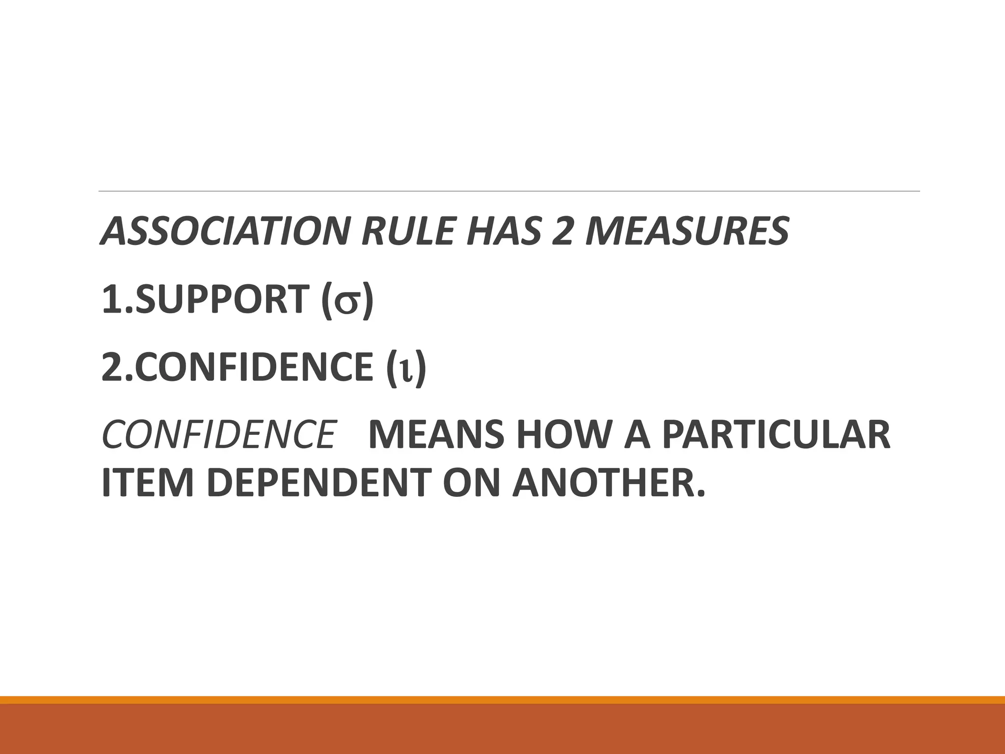
11. ASSOCIATION RULE HAS 2 MEASURES
1.SUPPORT ()
2.CONFIDENCE ()
CONFIDENCE MEANS HOW A PARTICULAR
ITEM DEPENDENT ON ANOTHER.

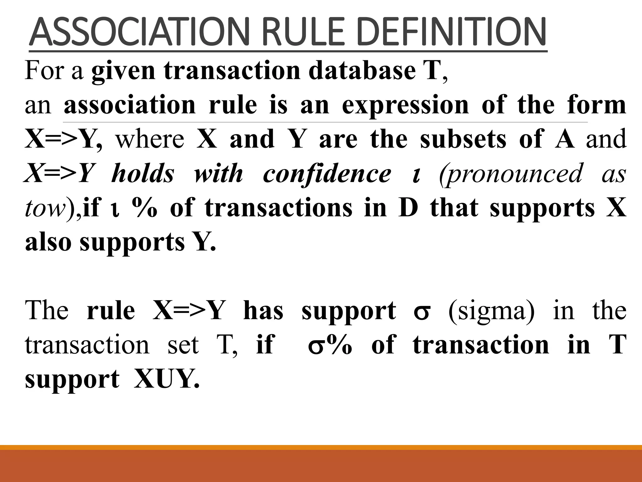
12. ASSOCIATION RULE DEFINITION
For a given transaction database T,
an association rule is an expression of the form
X=>Y, where X and Y are the subsets of A and
X=>Y holds with confidence  (pronounced as
tow),if  % of transactions in D that supports X
also supports Y.
The rule X=>Y has support  (sigma) in the
transaction set T, if % of transaction in T
support XUY.

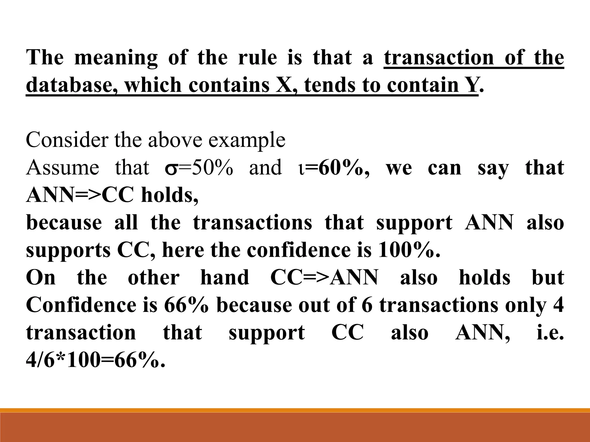
13. The meaning of the rule is that a transaction of the
database, which contains X, tends to contain Y.
Consider the above example
Assume that =50% and =60%, we can say that
ANN=>CC holds,
because all the transactions that support ANN also
supports CC, here the confidence is 100%.
On the other hand CC=>ANN also holds but
Confidence is 66% because out of 6 transactions only 4
transaction that support CC also ANN, i.e.
4/6*100=66%.

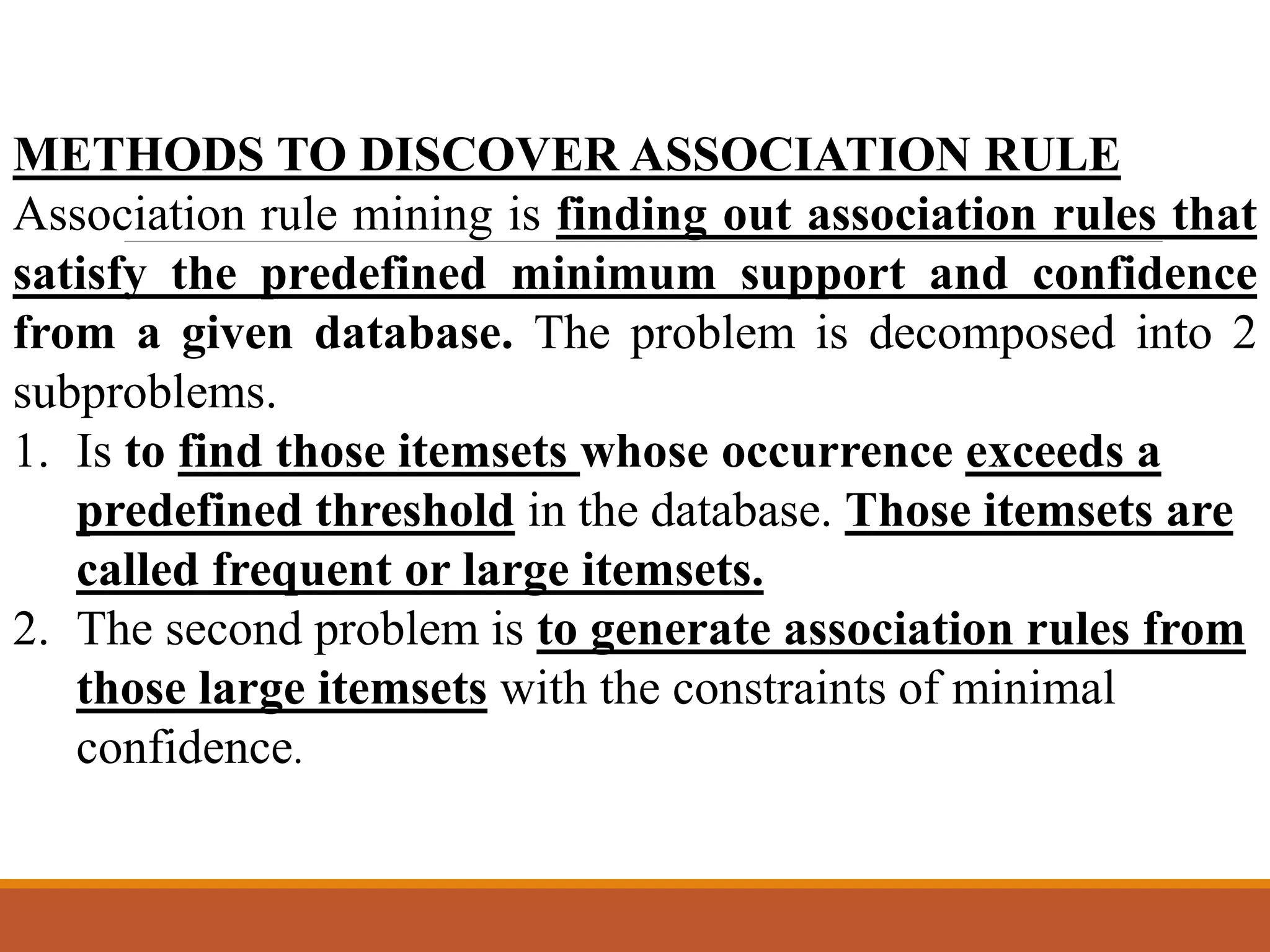
14. METHODS TO DISCOVER ASSOCIATION RULE
Association rule mining is finding out association rules that
satisfy the predefined minimum support and confidence
from a given database. The problem is decomposed into 2
subproblems.
1. Is to find those itemsets whose occurrence exceeds a
predefined threshold in the database. Those itemsets are
called frequent or large itemsets.
2. The second problem is to generate association rules from
those large itemsets with the constraints of minimal
confidence.

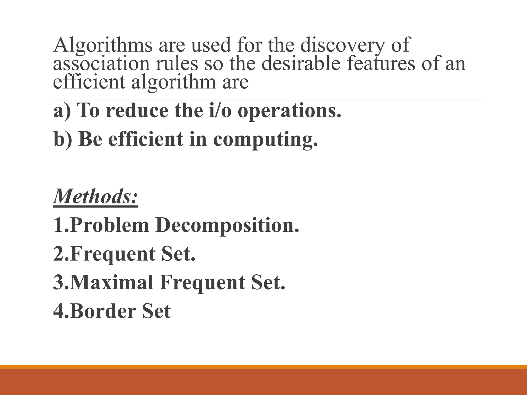
15. Algorithms are used for the discovery of
association rules so the desirable features of an
efficient algorithm are
a) To reduce the i/o operations.
b) Be efficient in computing.
Methods:
1.Problem Decomposition.
2.Frequent Set.
3.Maximal Frequent Set.
4.Border Set

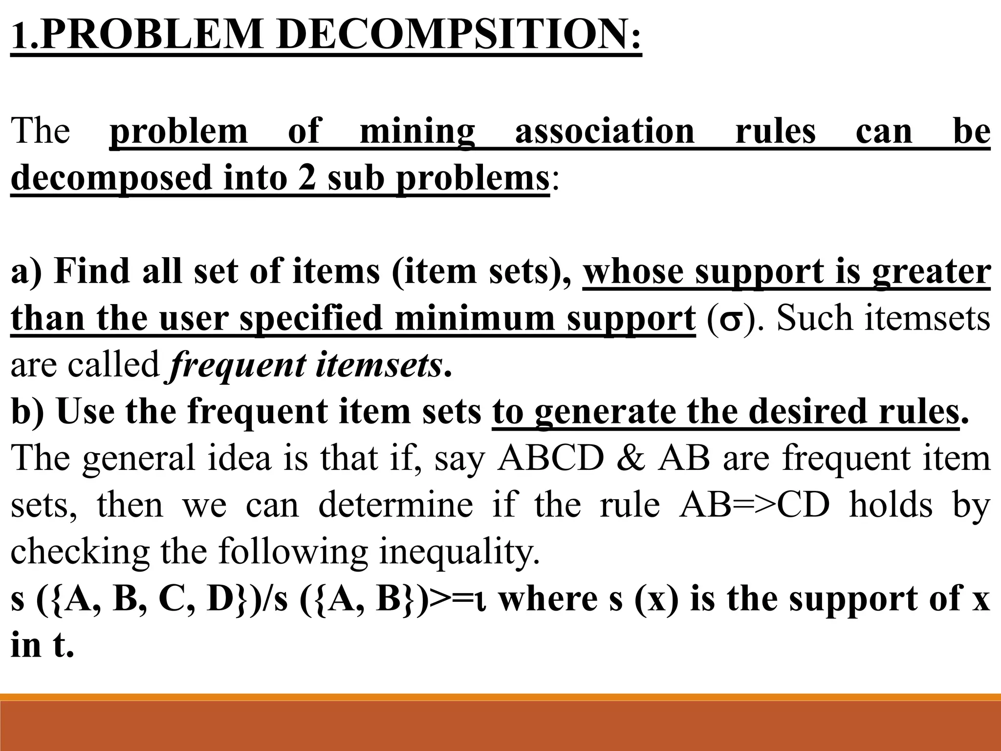
16. 1.PROBLEM DECOMPSITION:
The problem of mining association rules can be
decomposed into 2 sub problems:
a) Find all set of items (item sets), whose support is greater
than the user specified minimum support (). Such itemsets
are called frequent itemsets.
b) Use the frequent item sets to generate the desired rules.
The general idea is that if, say ABCD & AB are frequent item
sets, then we can determine if the rule AB=>CD holds by
checking the following inequality.
s ({A, B, C, D})/s ({A, B})>= where s (x) is the support of x
in t.

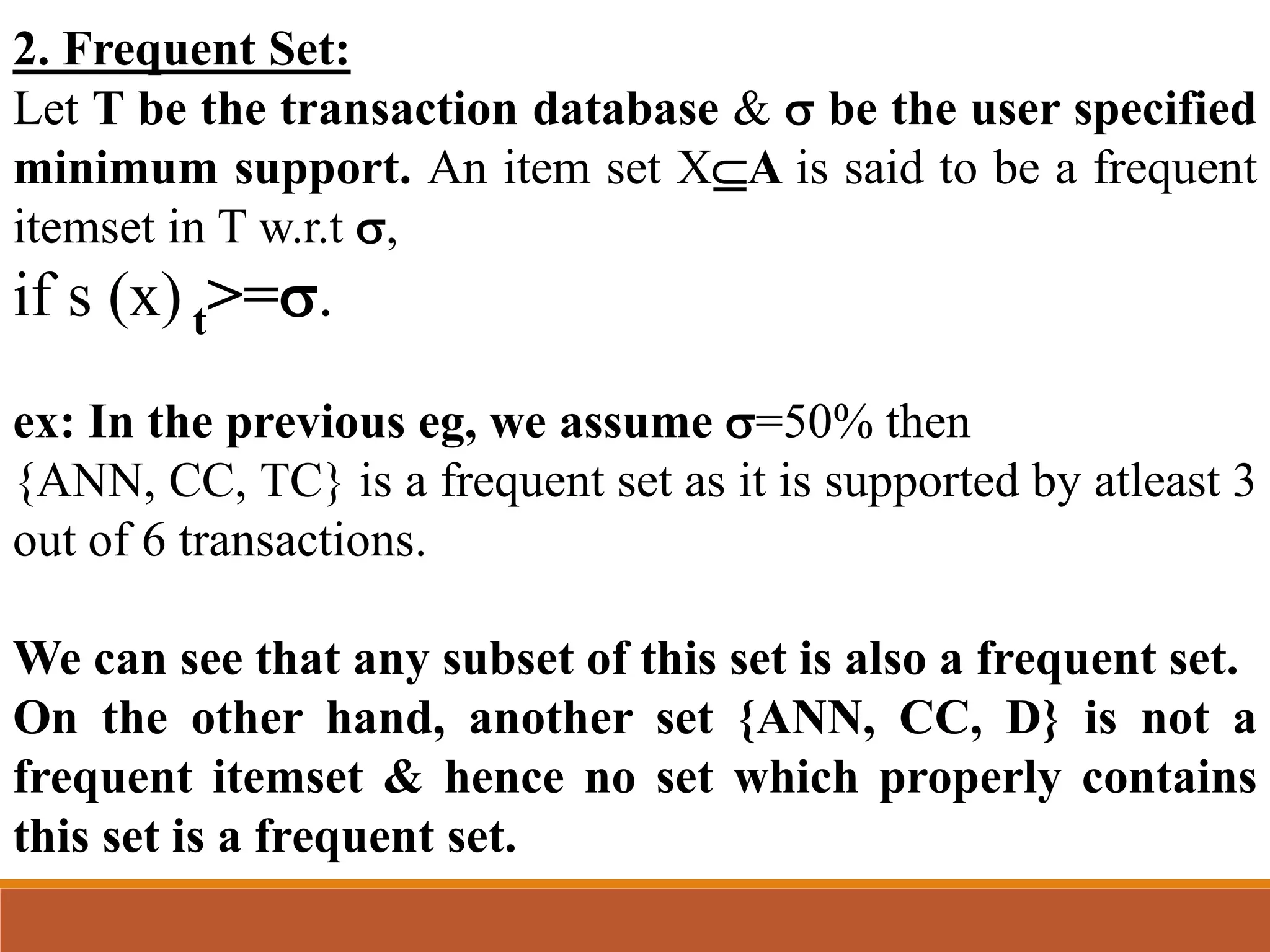
17. 2. Frequent Set:
Let T be the transaction database &  be the user specified
minimum support. An item set XA is said to be a frequent
itemset in T w.r.t ,
if s (x) t>=.
ex: In the previous eg, we assume =50% then
{ANN, CC, TC} is a frequent set as it is supported by atleast 3
out of 6 transactions.
We can see that any subset of this set is also a frequent set.
On the other hand, another set {ANN, CC, D} is not a
frequent itemset & hence no set which properly contains
this set is a frequent set.

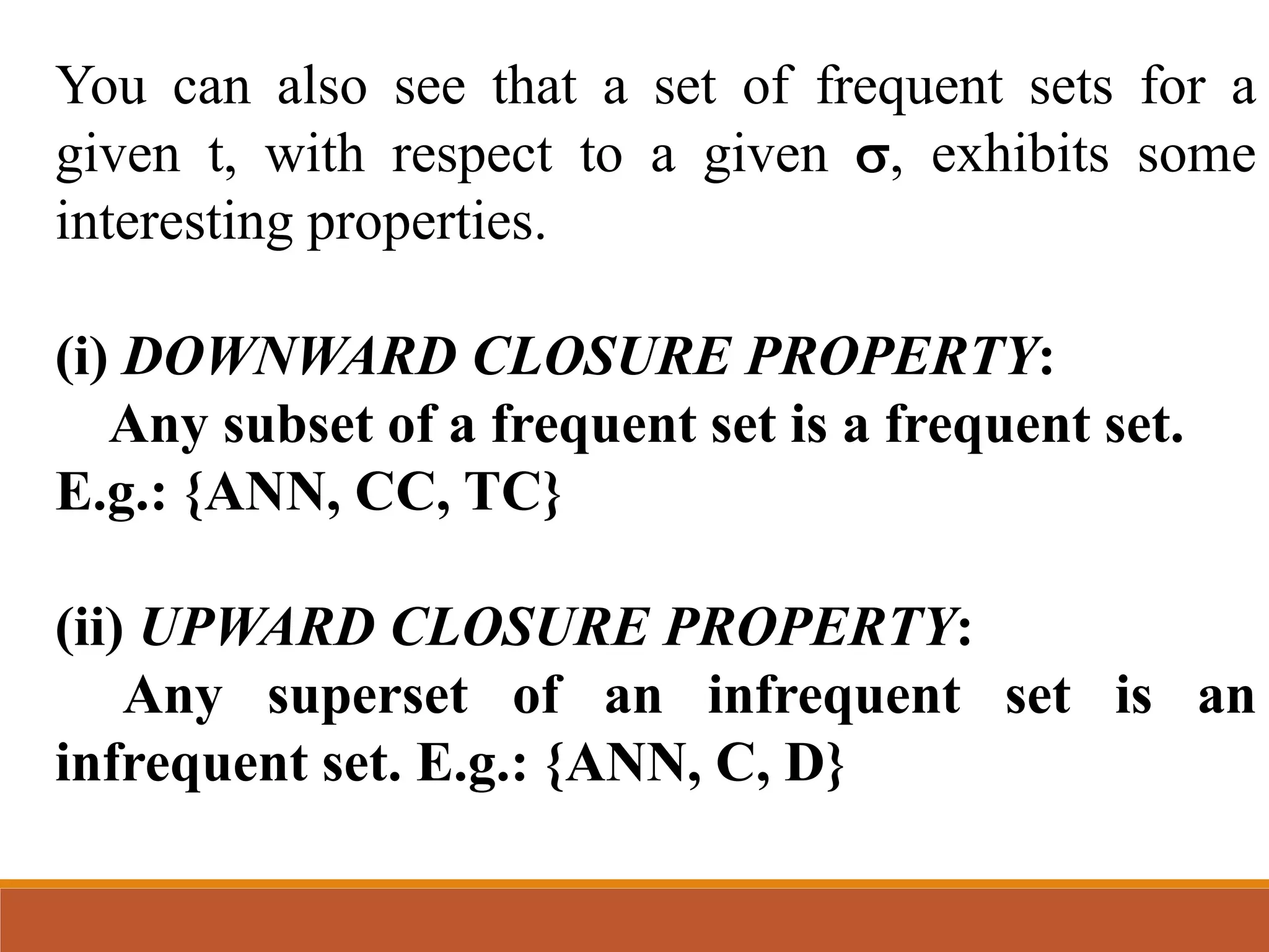
18. You can also see that a set of frequent sets for a
given t, with respect to a given , exhibits some
interesting properties.
(i) DOWNWARD CLOSURE PROPERTY:
Any subset of a frequent set is a frequent set.
E.g.: {ANN, CC, TC}
(ii) UPWARD CLOSURE PROPERTY:
Any superset of an infrequent set is an
infrequent set. E.g.: {ANN, C, D}

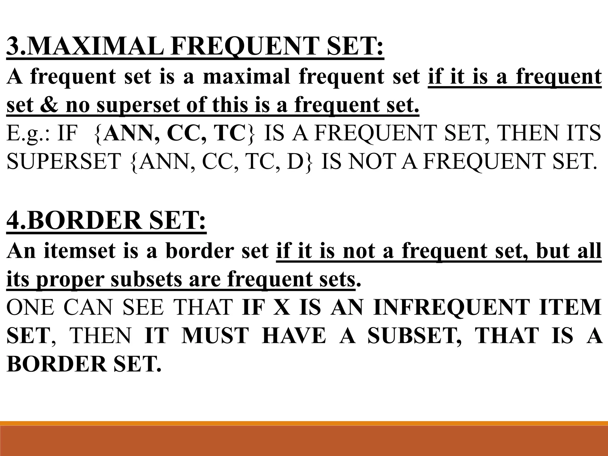
19. 3.MAXIMAL FREQUENT SET:
A frequent set is a maximal frequent set if it is a frequent
set & no superset of this is a frequent set.
E.g.: IF {ANN, CC, TC} IS A FREQUENT SET, THEN ITS
SUPERSET {ANN, CC, TC, D} IS NOT A FREQUENT SET.
4.BORDER SET:
An itemset is a border set if it is not a frequent set, but all
its proper subsets are frequent sets.
ONE CAN SEE THAT IF X IS AN INFREQUENT ITEM
SET, THEN IT MUST HAVE A SUBSET, THAT IS A
BORDER SET.

20. The Apriori Algorithm — Example
TID Items
100 1 3 4
200 2 3 5
300 1 2 3 5
400 2 5
Database D itemset sup.
{1} 2
{2} 3
{3} 3
{4} 1
{5} 3
itemset sup.
{1} 2
{2} 3
{3} 3
{5} 3
Scan D
C1
L1
itemset
{1 2}
{1 3}
{1 5}
{2 3}
{2 5}
{3 5}
itemset sup
{1 2} 1
{1 3} 2
{1 5} 1
{2 3} 2
{2 5} 3
{3 5} 2
itemset sup
{1 3} 2
{2 3} 2
{2 5} 3
{3 5} 2
L2
C2 C2
Scan D
C3 L3
itemset
{2 3 5}
Scan D itemset sup
{2 3 5} 2

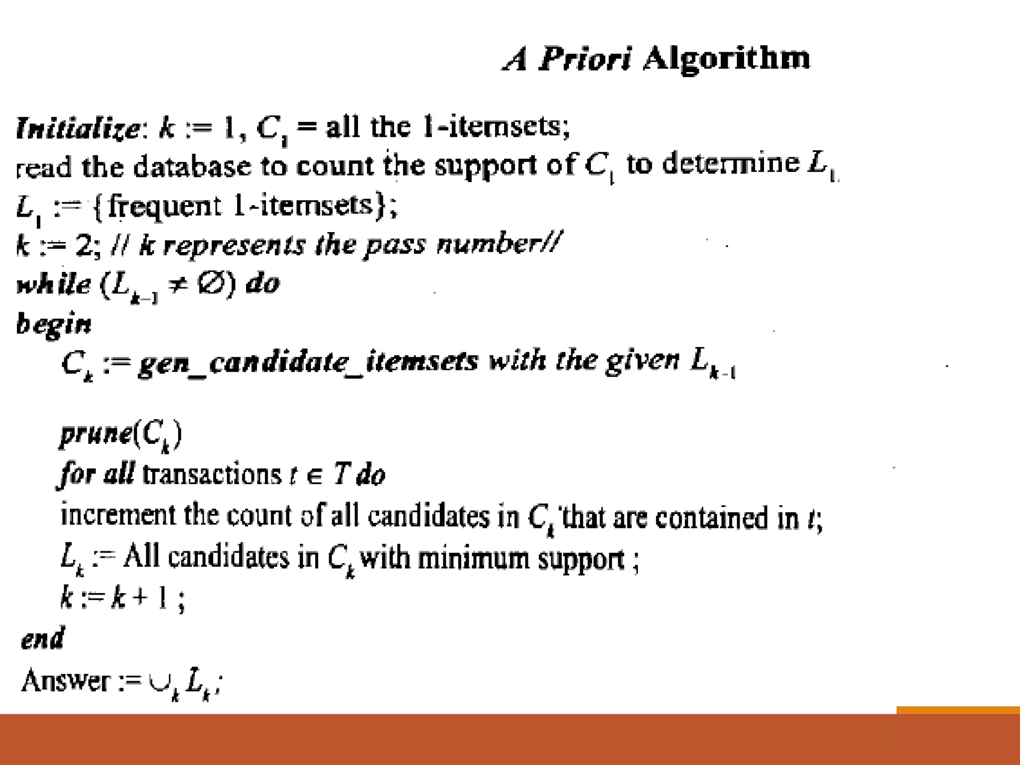
21. Apriori Algorithm
Also called as level wise algorithm. It was
proposed by Agarwal & Srikant in 1994.
It is the most popular algorithm to find all
frequent sets.
It makes use of downward closure property.
As the name suggest the algorithm is bottom up
search moving upward level wise in the lattice.

22. In order to implement this algorithm, 2 methods
are used i.e.,
1. The candidate generation process and
2. The pruning process are most important part of
this algorithm.

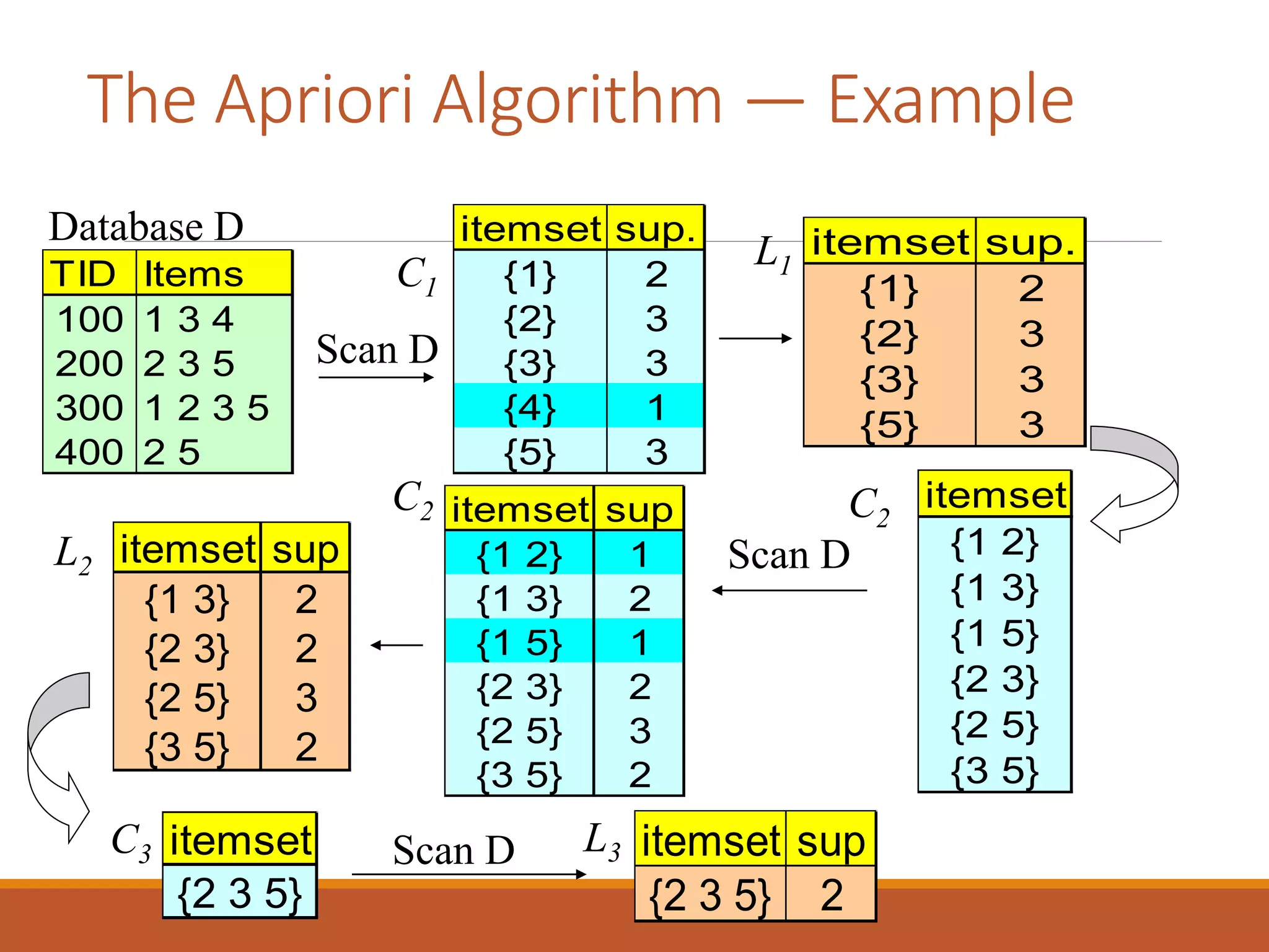
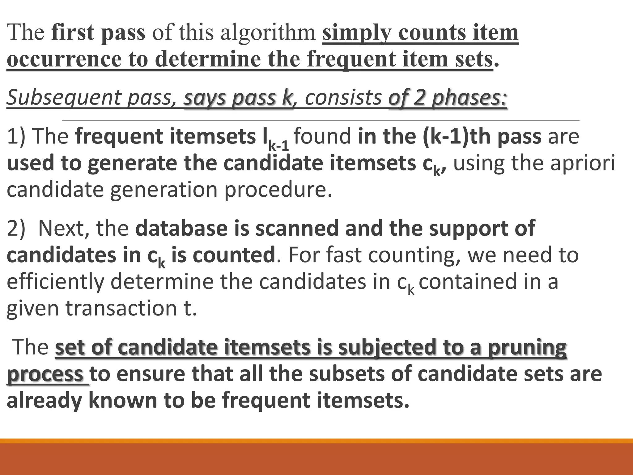
23. The first pass of this algorithm simply counts item
occurrence to determine the frequent item sets.
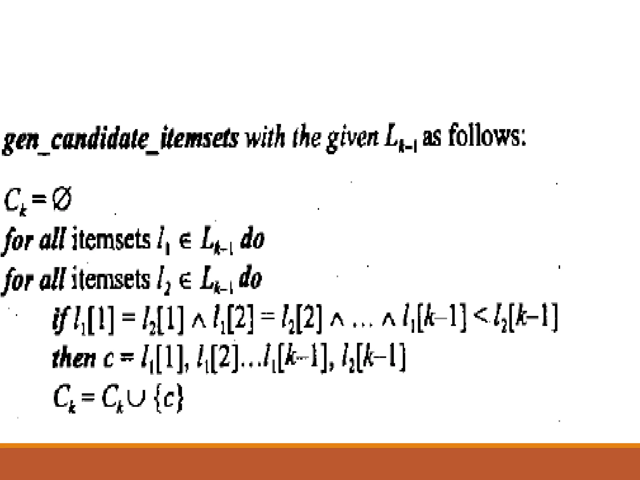
Subsequent pass, says pass k, consists of 2 phases:
1) The frequent itemsets lk-1 found in the (k-1)th pass are
used to generate the candidate itemsets ck, using the apriori
candidate generation procedure.
2) Next, the database is scanned and the support of
candidates in ck is counted. For fast counting, we need to
efficiently determine the candidates in ck contained in a
given transaction t.
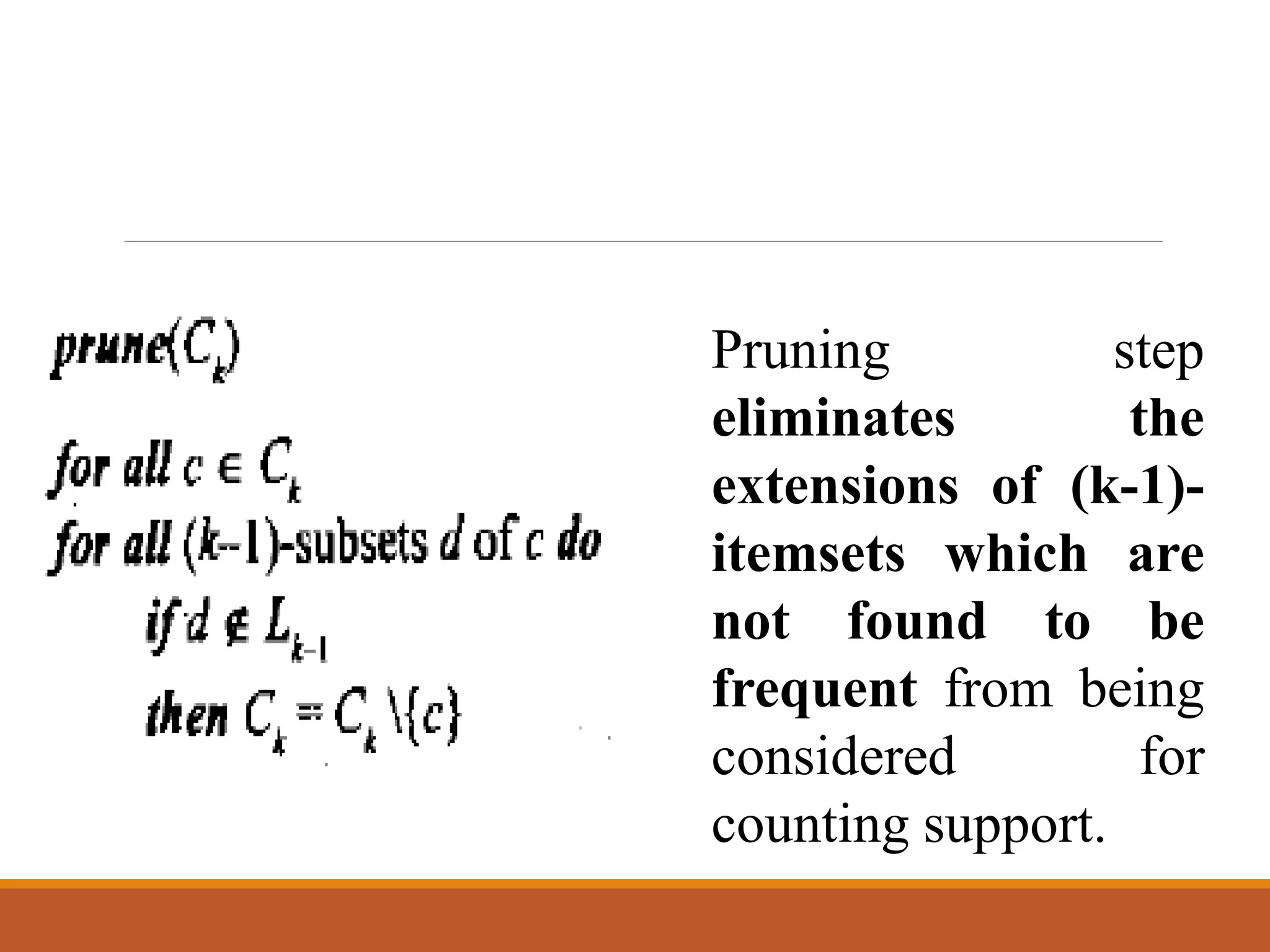
The set of candidate itemsets is subjected to a pruning
process to ensure that all the subsets of candidate sets are
already known to be frequent itemsets.

25. Pruning step
eliminates the
extensions of (k-1)-
itemsets which are
not found to be
frequent from being
considered for
counting support.

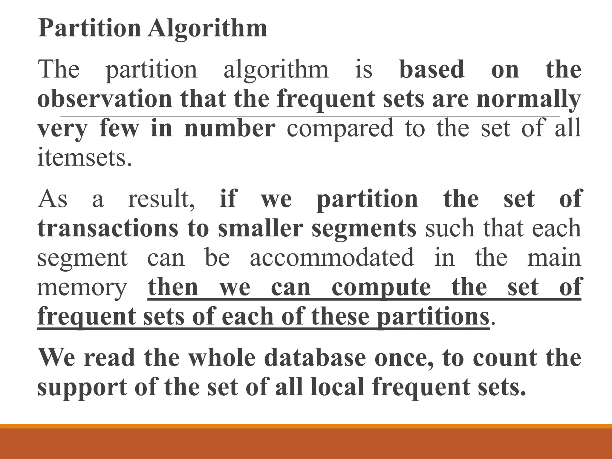
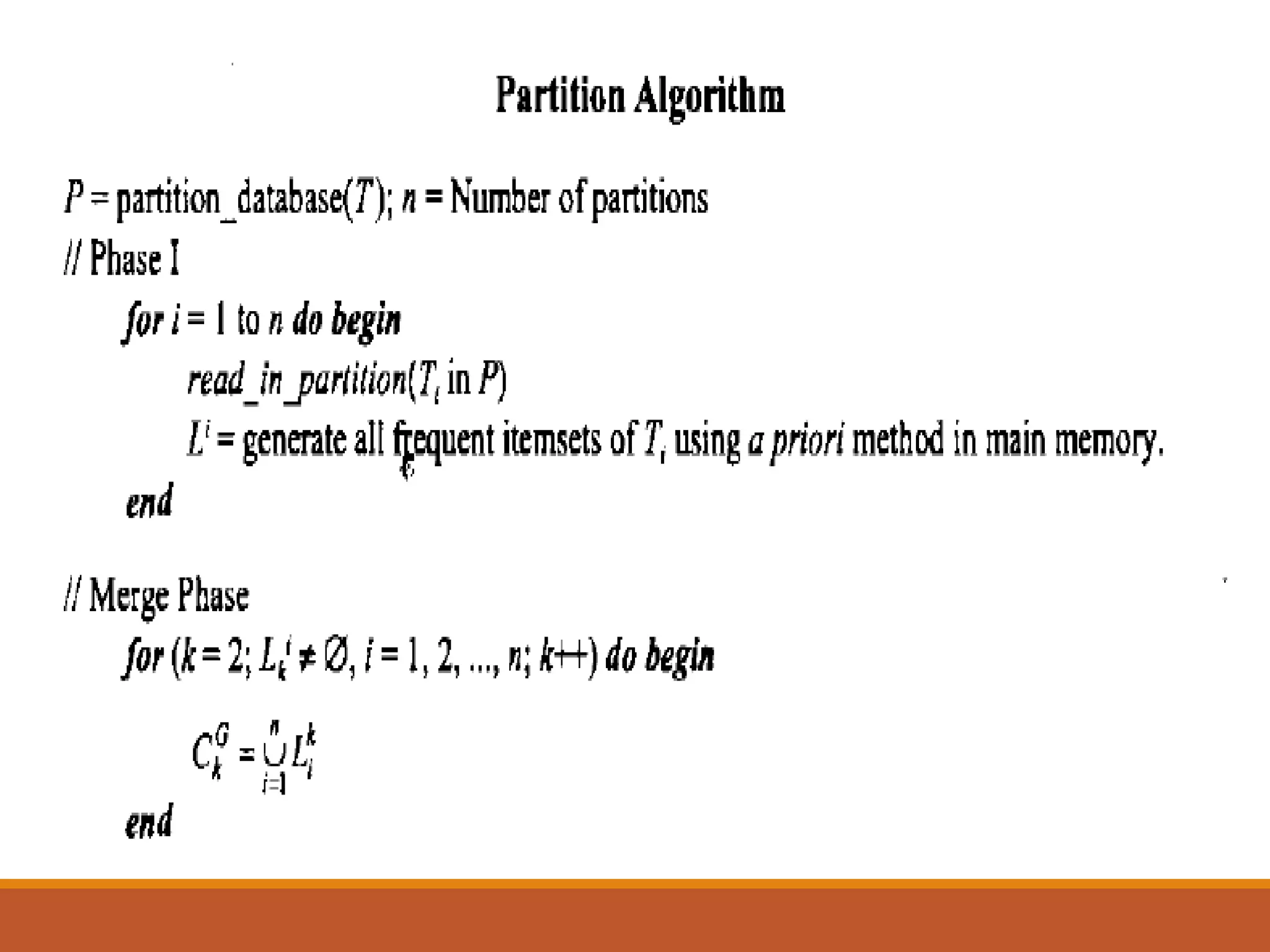
27. Partition Algorithm
The partition algorithm is based on the
observation that the frequent sets are normally
very few in number compared to the set of all
itemsets.
As a result, if we partition the set of
transactions to smaller segments such that each
segment can be accommodated in the main
memory then we can compute the set of
frequent sets of each of these partitions.
We read the whole database once, to count the
support of the set of all local frequent sets.

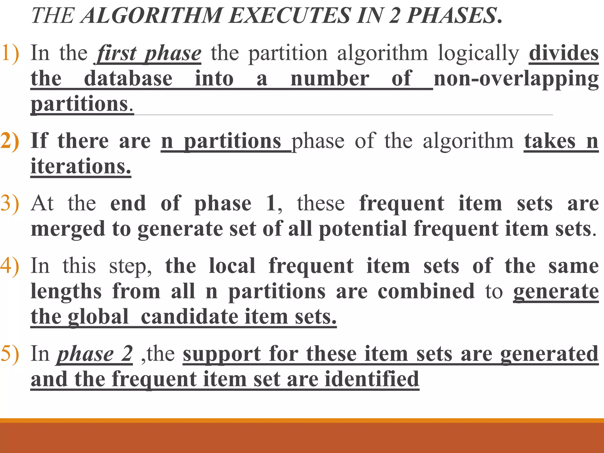
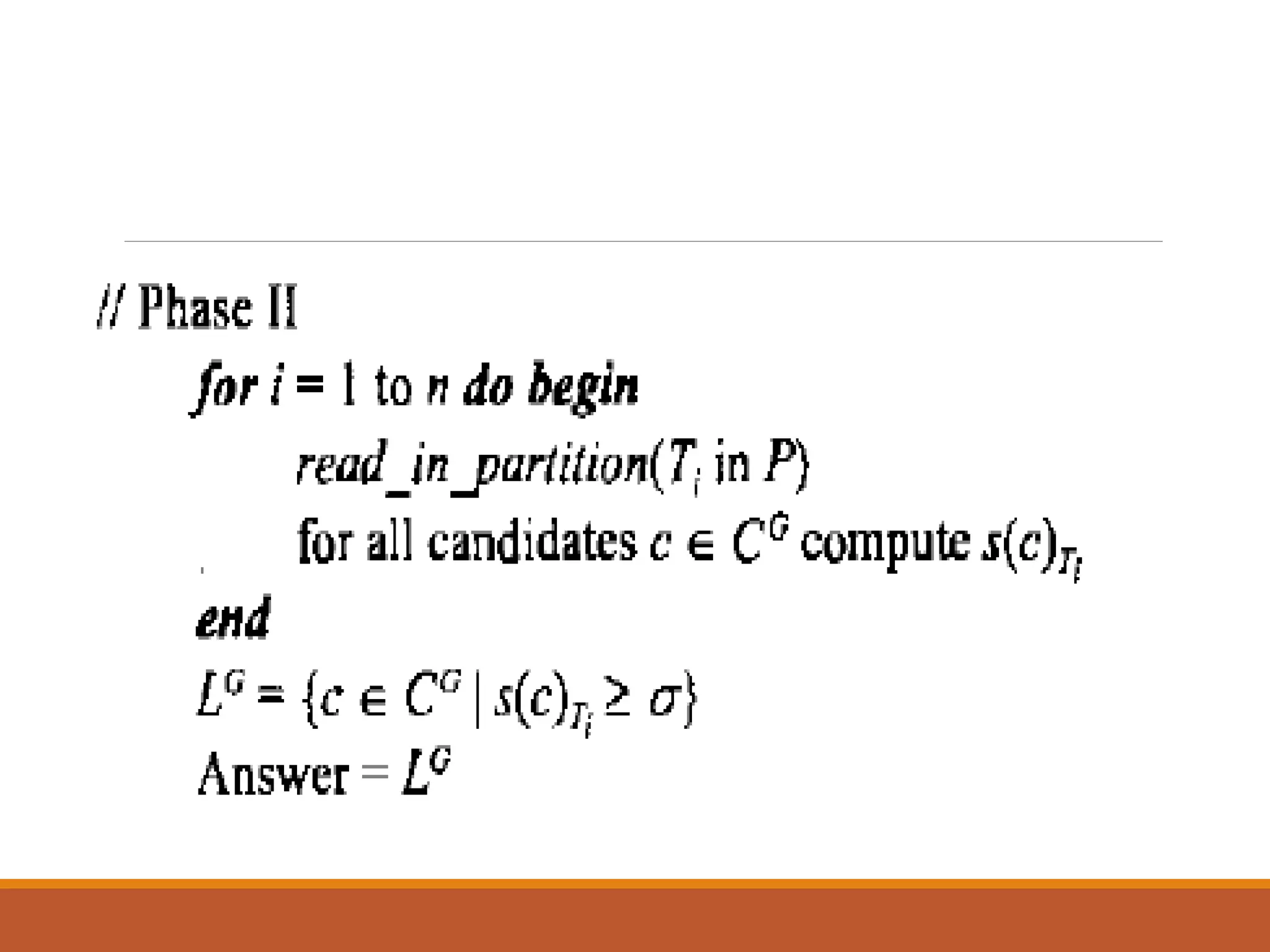
28. THE ALGORITHM EXECUTES IN 2 PHASES.
1) In the first phase the partition algorithm logically divides
the database into a number of non-overlapping
partitions.
2) If there are n partitions phase of the algorithm takes n
iterations.
3) At the end of phase 1, these frequent item sets are
merged to generate set of all potential frequent item sets.
4) In this step, the local frequent item sets of the same
lengths from all n partitions are combined to generate
the global candidate item sets.
5) In phase 2 ,the support for these item sets are generated
and the frequent item set are identified

32. Pincer-Search Algorithm
Pincer-Search Algorithm incorporates bi-directional search,
which takes advantage of both the bottom-up as well as the
top-down processes.
It attempts to find the frequent itemsets in a bottom-up
manner but at the same time, it maintains a list of maximal
frequent itemsets.
While making a database pass, it also counts the support of
these candidate maximal frequent itemsets to see if any one
of these is actually frequent. In that event, it can conclude that
all the subsets of these frequent sets are going to be frequent
and hence not verified for the support count in the next pass.
If we are lucky, we may discover a very large maximal
frequent itemset very early in this algorithm.

33. In this algorithm, in each pass, in addition to
counting the supports of the candidate in the
bottom-up direction,
it also counts the supports of the itemsets using
a top-down approach.
These are called the Maximal Frequent
Candidate Set (MFCS).
The process helps prune the candidate sets very
early on in the algorithm.
If we find a Maximal frequent set in this process, it
is recorded in the MFCS.

34. END