Hargreaves Class A method, Physical example, Christian sen method, estimation of evapotranspiration, PET, Methods of irrigation, Surface irrigation, free flooding irrigation method
This document discusses methods for calculating evaporation and return periods (recurrence intervals) for rainfall events. It provides an example of using the Weibull formula to calculate probabilities and return periods based on rainfall data from a station. The key steps are:
1) Arrange rainfall data in descending order.
2) Use the Weibull formula to calculate exceedance probabilities and return periods for each value.
3) Plot rainfall versus return period on semi-log paper to determine rainfall values for specified return periods.
4) Determine probability of an event equaling or exceeding a given rainfall amount by reading from the graph.
1) The document describes deriving a unit hydrograph from a storm hydrograph for a catchment area that experienced two rainfall events - a 3 cm storm followed by a 2 cm storm.
2) The resulting direct runoff hydrograph (DRH) is calculated using the principle of superposition, by combining the individual DRHs from each rainfall event at each time step.
3) The summary provides an example calculation of the 5 cm DRH at 3 hours, which is the sum of the 3 cm DRH (75 cm) and 2 cm DRH (0 cm) at that time.
Infiltration, aspects of infiltration, factors, measurement of infiltration, stream flow, infiltration indices, Discharge and measurement methods, Area-velocity and slope area methods, examples.infiltration,stream flow,
1. Specific energy is defined as the sum of the depth of flow and velocity head for a given discharge in an open channel. A specific energy curve relates the specific energy to the depth of flow for a particular channel section and discharge.
2. Local phenomena in open channels refer to rapid changes from subcritical to supercritical flow and vice versa, resulting in changes from high stage to low stage. The two types of local phenomena are hydraulic drops and hydraulic jumps.
3. A hydraulic drop is a steep depression in the water surface caused by an abrupt change in channel slope or cross section. A hydraulic jump is a rapid rise in the water surface caused by a transition from low stage to high stage.
The document describes methods for calculating river discharge, including the area-velocity method and slope-area method. The area-velocity method divides the river cross section into segments, calculates the average width and velocity for each, and sums the segmental discharges. The slope-area method estimates discharge over a long reach based on the high flood level, total flow area, slope of the water surface, and whether the reach is contracting or expanding.
Velocity distribution, coefficients, pattern of velocity distribution,examples, velocity measurement, derivation of velocity distribution coefficients, problems and solution, Bernoulli's theorem and energy equation, specific energy and equation.
The document discusses flow properties in open channels including:
- The Reynolds number and Froude number, which characterize flow regimes as turbulent or laminar and subcritical/supercritical.
- Hydraulic properties such as depth, area, wetted perimeter, hydraulic radius, and section factor which describe channel geometry.
- Critical flow occurs when the Froude number equals 1. Subcritical flow has a Froude number less than 1 while supercritical flow has a Froude number greater than 1.
- Examples are provided to demonstrate calculating hydraulic properties for given channel cross sections.
This document discusses different methods for computing average rainfall over a basin including arithmetic average, Thiessen polygon, and isohyetal methods. It provides examples of calculating average rainfall using each method. It also discusses presenting rainfall data through mass curves and hyetographs. The arithmetic average method simply takes the mean of recorded rainfall values at stations. Thiessen polygon method weights values based on each station's representative area. Isohyetal mapping involves contouring equal rainfall and calculating weighted averages between contours.
This document summarizes methods for flood probability analysis and flood frequency analysis. It discusses obtaining flood records, ranking floods by exceedance probability, and plotting the data on probability charts. It also describes regional flood frequency analysis using regional curves, and synthetic unit hydrograph methods for estimating floods in ungauged basins based on geometric properties.
This document describes how to derive a required time (T) unit hydrograph from a given time (D) unit hydrograph when T is not a multiple of D using the S-curve method. It explains that an S-curve hydrograph is generated by continuous, uniform effective rainfall and rises continuously in the shape of an S until equilibrium is reached. The ordinates of the S-curve can be calculated using the equation S(t) = U(t) + S(t-D), where S(t) is the ordinate of the S-curve at time t, U(t) is the ordinate of the given unit hydrograph at time t, and S(t-D) is the
This presentation summarizes key concepts related to hydrographs including:
1) A hydrograph shows the variation of discharge over time at a particular point in a river. It has three main components: the rising limb, peak, and recession curve.
2) Factors like area, slope, land use, and precipitation affect hydrograph shape.
3) A unit hydrograph represents the response of a watershed to 1 cm of direct runoff from rainfall of a given duration, and is used to estimate flood discharge from future rainfall.
4) Methods like superposition and S-curves are used to derive unit hydrographs from storm hydrographs and to estimate hydrographs for different rainfall scenarios.
The document discusses unit hydrographs and their applications in flood prediction. A unit hydrograph models the runoff response of a watershed to one inch of excess rainfall over a given duration. It can be used to predict the runoff hydrograph from a storm of any size by applying the principles of superposition and proportionality. The key steps in developing a unit hydrograph involve analyzing rainfall and runoff data from a storm event to separate baseflow, calculating the volume of excess runoff, and adjusting the hydrograph to represent the response to one inch of rainfall.
This document describes Snyder's synthetic unit hydrograph method. Snyder's method allows computation of key hydrograph characteristics using watershed properties. These include:
1. Lag time, which is related to watershed time of concentration based on length and slope.
2. Hydrograph duration, which is typically 1/5.5 of the lag time.
3. Peak discharge, which is related to watershed area, storage coefficient, and time parameters.
4. Other hydrograph properties like width can also be estimated using the peak discharge and empirical coefficients. The synthetic hydrograph provides an estimate of watershed runoff for both gauged and ungauged locations.
This document discusses methods for estimating peak or flood discharge in rivers. It describes 6 main approaches: 1) Using physical conditions from past floods, 2) Flood discharge formulae based on catchment area, 3) Flood frequency studies using probability concepts, 4) The unit hydrograph method, 5) The rational formula, and 6) The modified rational formula which includes a storage coefficient. Examples are provided for each method to illustrate how to estimate peak discharge values.
This document provides an introduction to flood frequency analysis, which uses historical flood data to estimate the probability and recurrence intervals of future floods of given magnitudes. It discusses how flood frequency analysis is necessary for cost-effective design of bridges, dams, and other structures, as well as flood insurance and zoning. Two common methods for collecting flood data are described: annual peaks and partial duration series. Statistical approaches like the Weibull formula are commonly used to analyze the data and construct flood frequency curves showing the relationship between discharge magnitude and probability or recurrence interval.
The document discusses unit hydrographs, which are used to model the response of a watershed's streamflow to rainfall. It covers topics such as:
- Defining a unit hydrograph and explaining its use in predicting streamflow from rainfall amounts.
- Describing the assumptions and terminology used in unit hydrograph models, such as uniform rainfall distribution and the components of a hydrograph.
- Explaining how to create a unit hydrograph from streamflow data or synthetically, and how to apply it to calculate a direct runoff hydrograph from rainfall inputs.
This document discusses moist processes in meteorology. It explains that water vapor makes up most of the water in the atmosphere and exists primarily in the troposphere. Condensation occurs when air is cooled to below its dew point, through processes like lifting, mixing with cooler air masses, or contact cooling over surfaces. Lifting air parcels cools them through expansion, with the lifting condensation level being reached when the air reaches saturation. Further lifting causes additional condensation as more water vapor condenses out of the rising air parcel. This condensation releases latent heat, slowing the cooling rate compared to unsaturated air parcels. The document also describes how downslope winds like Föhn winds can warm as they descend,
This document discusses air pressure and moisture. It defines air pressure as the force of air pressing down on Earth's surface, which depends on air density. Factors that affect air pressure include temperature, water vapor, and elevation. As elevation increases, air becomes less dense and pressure decreases. Air pressure is measured using barometers like mercury or aneroid barometers. Relative humidity describes the amount of water vapor in air compared to the maximum it could hold at a given temperature, and is measured using a psychrometer. Higher relative humidity means slower evaporation.
1) Atmospheric pressure is caused by the weight of air molecules pressing down on surfaces below. The random motion of air molecules propagates this pressure equally in all directions.
2) Atmospheric pressure is measured using a mercury barometer, with standard atmospheric pressure at sea level being approximately 1013 hPa. Global maps of current sea-level air pressure show values typically between 1005-1047 hPa.
3) Pressure gradients are weak near the Earth's surface because winds act to reduce differences in pressure over time, transporting air from high to low pressure areas.
The document discusses precipitation measurement and analysis. It defines precipitation as water that reaches the earth from the atmosphere in forms such as rainfall, snowfall, hail, etc. Rainfall is the predominant form and is measured using rain gauges, which can be non-recording or recording. Rainfall data is analyzed spatially over areas using methods like Thiessen polygons to determine average rainfall over a catchment from point measurements. Temporal variation in rainfall is also examined from hourly to annual scales to understand precipitation patterns.
The document contains a practice test for the IESO 2012 Written TEST Atmosphere and Hydrosphere. It includes 14 multiple choice questions about atmospheric and oceanographic concepts, figures, and calculations. Key topics covered include the tropopause, jet streams, pressure systems, fronts, clouds, humidity, the hydrostatic equation, and ocean mixed layers and thermoclines. The test evaluates understanding of scientific diagrams, definitions, and the ability to perform calculations related to meteorology and physical oceanography.
The document discusses various components of weather including:
1. Uneven heating of the Earth's atmosphere by the sun causes air movements and reactions that produce the wide variety of weather conditions.
2. Key weather variables such as temperature, air pressure, moisture, wind speed and direction are measured using instruments like thermometers, barometers, and anemometers.
3. Moisture in the atmosphere exists as water vapor, liquid droplets, or ice crystals, and the amount of moisture the air can hold depends on temperature. Changes in temperature and moisture can lead to precipitation.
Humidity refers to the amount of water vapor in the air. It is measured by relative humidity and dew point temperature. Condensation occurs when warm, moist air rises and cools, causing water vapor to condense into liquid water droplets. The main types of precipitation are rain, snow, sleet, hail, and drizzle, which occur via different meteorological processes like convection, orographic lifting, and frontal lifting. Thunderstorms occur when upward motion within clouds causes water droplets to collide and become electrified.
The document discusses hydrological losses and factors affecting evaporation. It defines different types of hydrological losses including interception, depression storage, evaporation, transpiration, and infiltration. It then discusses various meteorological parameters that influence the evaporation process such as temperature, humidity, wind, radiation, and atmospheric pressure. Temperature affects evaporation rate but not always proportionally. Humidity and vapor pressure influence the vapor pressure deficit which governs evaporation rate. Wind helps carry away moisture and accelerates evaporation up to a critical speed. The nature of the evaporating surface like soil moisture levels also impacts evaporation rate.
This document defines meteorological terms and describes the vertical structure of Earth's atmosphere. It discusses:
1. The layers of the atmosphere including the troposphere, stratosphere, and mesosphere. The troposphere is where weather occurs and has decreasing temperature with altitude.
2. The boundary layer, a sublayer of the troposphere directly influenced by surface friction and turbulence.
3. Temperature and pressure decrease logarithmically with altitude. Horizontal gradients are generally much smaller than vertical gradients.
4. Time is usually reported in UTC and units include Kelvin, Celsius, Fahrenheit for temperature and millibars, Pascals for pressure.
Atmospheric pressure decreases with increasing altitude due to less air above. The barometric formula models how pressure and density change with altitude, dropping off exponentially. At sea level, air has a density of about 1.2 kg/m3 under standard temperature and pressure, but density decreases with altitude as pressure and temperature drop under the effects of gravity and the dry adiabatic lapse rate.
This document outlines chapter 5 on air pollution meteorology. It discusses key meteorological concepts that influence the dispersion of air pollutants, including solar radiation, atmospheric pressure, lapse rates, atmospheric stability, Coriolis force, and gravitational force. Homework assignments are provided asking students to research and calculate values related to these topics to better understand atmospheric conditions and pollutant transport.
Metfi 120 (introduction to Weather and Climato) Orline - Unit 2 Revie.pdfamericandigitalshop
Metfi 120 (introduction to Weather and Climato) Orline - Unit 2 Review Adiabatic processes in
the mountaln. The diagram below shows the lapse rates that air parcel will encounter while it is
forced to move over a mountain. If an alr parcel descends through the atmosphere the air will
heat at the dry adiabatic rate as it will necessarily be unsaturated. In summary, while rising air
cools at varying rates, descending air heats at a uniform rate. 16. Using the table below, fill in the
blanks for temperature and dew-point temperature at various helghts on the windward and
leeward sides of the mountain. Assume that the WALR is 0.5C/100m. (Note: temperature and
dew-paint drop together above LCL when a saturated air parcel rises and water vapor condonses.
In addition, start from the 500m at windward side 1000m1500m2000m Peak 2000m at leeward
side 1500m1000m500m Sea Level at leeward side.) 17. Compare to those of on the windward
side, how do air temperature and dew point on the leeward side? 18. From the previous question,
Why?
MEIR120 (introduction to Weather and CImate) Onine - Unit2 Review Here is a challenging
question. Assume that the wet adiabatic lapse rate (WALR) is 0.6C/100m. Fill the blanks in the
boxes in the figure. Here is how to get answers. 1. At the LCL, temperature (2C) and dew point
(2C) are the same. Until air parcel reaches LCL, temperature falls at the DALR (1.0C/100m). At
the LCL, temperature falls 25C from the surface (27C2C=25C). It means air parcel rises 2500m.
Thus LCL is 2500m. 2. Below the LCL, dew point changes at the Dew Point Lapse Rate (DPLR,
0.2C/100m ), it means that dew point has changed 5.0C(0.2C/100m2500m). Thus dew point at
the surface is 7C/100m 3. Above the LCL, both temperature and dew point fall at the WALR
(0.6C/100m). Atthe peak, dew point is 1C. It is 3C cooler than the LCL. It means air parcel rises
another 500m(0.6C/100m500m=3C). Thus, peak elevation is
3000m(LCL+500m=2500m+500m) 4. At the leeward side, temperature and dew point rise at the
DALR (1.0C/100m) and DPLR (0.2C/100m), respectively. Elevation has changed
2500m(3000m500m). Thus temperature and dew point rise 25C/100m and 5C. Thus, temperature
will be 24C(1C+25C) and dew point will be 4C(1C+5C).
Chapter 6: Precipitation and its formation Steps in the formation of precipitation according to the
Bergeron process. The Bergeron process relies on the fact that cloud droplets do not freeze until
they reach a temperature below the freezing point, and even then only in the presence of freezing
nuclei (solid particles that have a crystal form similar to that of ice). Because freezing nuclel are
much less abundant than condensation nuclei, many clouds exist in the liquid state while at
temperatures well below 0C. These are supercooled clouds. The freezing nuclei present promote
the formation of a few scattered ice crystals. Since lce crystals are more efficient absorbers of
water vapor, they consume the "excess" water vapor, which lowers the relative humid.
The document discusses various weather and climate concepts including:
- Weather is the current atmospheric conditions while climate is the average weather over time.
- High pressure systems are associated with clear skies and dry conditions while low pressure systems bring clouds and rain.
- Weather maps use lines of equal pressure (isobars) and symbols to show wind speed and direction helping predict future conditions.
This document discusses the standard atmosphere and how atmospheric pressure varies with altitude. It provides information on how pressure decreases as altitude increases, dropping about 1.2 kPa for every 100 meters at low altitudes. The document also presents an equation called the barometric formula that relates atmospheric pressure, altitude, temperature, and other parameters in the troposphere. It includes a table with typical values for these parameters.
The document discusses meteorological parameters that influence air quality and dispersion modeling. Primary parameters include wind speed, direction, and atmospheric stability, while secondary parameters include temperature, precipitation, and topography. Atmospheric stability is determined by comparing the ambient lapse rate to the dry adiabatic lapse rate. Stability categories include unstable, neutral, and stable atmospheres. Plume rise and dispersion are influenced by stability, with unstable air resulting in greater vertical mixing and stable air suppressing vertical dispersion. The Gaussian plume model is presented as a method to estimate pollutant concentrations downwind of a point source.
CAMBRIDGE AS GEOGRAPHY REVISION: ATMOSPHERE AND WEATHER - 2.1 LOCAL ENERGY BU...George Dumitrache
A comprehensive presentation of subchapter 2.1 Local Energy Budgets, from the second chapter of Physical Geography, AS Cambridge, Atmosphere and Weather.
This chapter discusses how meteorological conditions influence the transport and dispersion of air pollutants. It covers key topics such as:
1) Wind patterns from global to micro scales that affect pollutant movement.
2) Lapse rates which describe how temperature changes with altitude. Inversions and stable/unstable conditions impact vertical air movement.
3) Maximum mixing depth, the vertical extent of mixing which influences pollutant dispersion and urban air pollution episodes.
This document discusses how meteorological conditions influence the transport and dispersion of air pollutants. It covers topics such as wind patterns from macro to micro scales; lapse rates and their relationship to atmospheric stability; types of inversions like subsidence and radiation inversions; and the maximum mixing depth which determines the vertical extent of pollutant dispersion. Diagrams are included to illustrate concepts like wind profiles, wind roses, stability conditions, and mixing depths.
This chapter discusses how meteorological conditions influence the transport and dispersion of air pollutants. It covers key topics such as:
1) Wind patterns from global to micro scales that determine pollutant movement.
2) Lapse rates which describe how temperature changes with altitude. Inversions and stable/unstable conditions impact vertical mixing.
3) Maximum mixing depth, the vertical extent of mixing which affects pollutant dispersion and influences air quality.
Similar to Class lectures on Hydrology by Rabindra Ranjan Saha Lecture 2 (20)
Vision & Mission, Course profile, :Lesson Plan, Definition on hydrology, hydrologic cycle, uses of hydrology, solar and earth radiation, temperature, measurement of radiation, vapor.
The document describes various methods of irrigation including check flooding, basin flooding, furrow irrigation, subsurface irrigation, sprinkler irrigation, and drip/trickle irrigation. Check flooding involves enclosing level plots with small levees and flooding the enclosed area with irrigation water. Basin flooding is a type of check flooding used for orchard trees, with one or more trees placed in flooded basins. Furrow irrigation involves creating small parallel channels for water to flow down the field. Subsurface irrigation applies water from beneath the soil surface using trenches or perforated pipes. Sprinkler irrigation sprays water into the air to break into small drops and fall to the ground, similar to natural rainfall. Drip/trickle irrigation slowly applies water
The document discusses different sources of irrigation water including rainfall, surface water sources like rivers and lakes, groundwater sources like shallow wells, and combinations of surface and groundwater. It describes factors to consider for different water sources like quantity needs, quality, and competing uses. Water quality parameters for irrigation include electrical conductivity, sodium absorption ratio, and concentrations of salts, sodium, calcium, magnesium, and toxic elements. The document provides classifications for water salinity levels and sodium hazards and their suitability for irrigation on different soil types.
Open channel Flow -Class lectures at WUB, Book references, Mission and Vision, CO and PO, definition of OCF, Aplication of Hydraulics, ,Difference between OCF and Pipe flow, Classification, Flow profile and cross sections.
Applications of artificial Intelligence in Mechanical Engineering.pdfAtif Razi
Historically, mechanical engineering has relied heavily on human expertise and empirical methods to solve complex problems. With the introduction of computer-aided design (CAD) and finite element analysis (FEA), the field took its first steps towards digitization. These tools allowed engineers to simulate and analyze mechanical systems with greater accuracy and efficiency. However, the sheer volume of data generated by modern engineering systems and the increasing complexity of these systems have necessitated more advanced analytical tools, paving the way for AI.
AI offers the capability to process vast amounts of data, identify patterns, and make predictions with a level of speed and accuracy unattainable by traditional methods. This has profound implications for mechanical engineering, enabling more efficient design processes, predictive maintenance strategies, and optimized manufacturing operations. AI-driven tools can learn from historical data, adapt to new information, and continuously improve their performance, making them invaluable in tackling the multifaceted challenges of modern mechanical engineering.
Mechatronics is a multidisciplinary field that refers to the skill sets needed in the contemporary, advanced automated manufacturing industry. At the intersection of mechanics, electronics, and computing, mechatronics specialists create simpler, smarter systems. Mechatronics is an essential foundation for the expected growth in automation and manufacturing.
Mechatronics deals with robotics, control systems, and electro-mechanical systems.
Software Engineering and Project Management - Software Testing + Agile Method...Prakhyath Rai
Software Testing: A Strategic Approach to Software Testing, Strategic Issues, Test Strategies for Conventional Software, Test Strategies for Object -Oriented Software, Validation Testing, System Testing, The Art of Debugging.
Agile Methodology: Before Agile – Waterfall, Agile Development.
DEEP LEARNING FOR SMART GRID INTRUSION DETECTION: A HYBRID CNN-LSTM-BASED MODELijaia
As digital technology becomes more deeply embedded in power systems, protecting the communication
networks of Smart Grids (SG) has emerged as a critical concern. Distributed Network Protocol 3 (DNP3)
represents a multi-tiered application layer protocol extensively utilized in Supervisory Control and Data
Acquisition (SCADA)-based smart grids to facilitate real-time data gathering and control functionalities.
Robust Intrusion Detection Systems (IDS) are necessary for early threat detection and mitigation because
of the interconnection of these networks, which makes them vulnerable to a variety of cyberattacks. To
solve this issue, this paper develops a hybrid Deep Learning (DL) model specifically designed for intrusion
detection in smart grids. The proposed approach is a combination of the Convolutional Neural Network
(CNN) and the Long-Short-Term Memory algorithms (LSTM). We employed a recent intrusion detection
dataset (DNP3), which focuses on unauthorized commands and Denial of Service (DoS) cyberattacks, to
train and test our model. The results of our experiments show that our CNN-LSTM method is much better
at finding smart grid intrusions than other deep learning algorithms used for classification. In addition,
our proposed approach improves accuracy, precision, recall, and F1 score, achieving a high detection
accuracy rate of 99.50%.
Optimizing Gradle Builds - Gradle DPE Tour Berlin 2024Sinan KOZAK
Sinan from the Delivery Hero mobile infrastructure engineering team shares a deep dive into performance acceleration with Gradle build cache optimizations. Sinan shares their journey into solving complex build-cache problems that affect Gradle builds. By understanding the challenges and solutions found in our journey, we aim to demonstrate the possibilities for faster builds. The case study reveals how overlapping outputs and cache misconfigurations led to significant increases in build times, especially as the project scaled up with numerous modules using Paparazzi tests. The journey from diagnosing to defeating cache issues offers invaluable lessons on maintaining cache integrity without sacrificing functionality.
Null Bangalore | Pentesters Approach to AWS IAMDivyanshu
#Abstract:
- Learn more about the real-world methods for auditing AWS IAM (Identity and Access Management) as a pentester. So let us proceed with a brief discussion of IAM as well as some typical misconfigurations and their potential exploits in order to reinforce the understanding of IAM security best practices.
- Gain actionable insights into AWS IAM policies and roles, using hands on approach.
#Prerequisites:
- Basic understanding of AWS services and architecture
- Familiarity with cloud security concepts
- Experience using the AWS Management Console or AWS CLI.
- For hands on lab create account on [killercoda.com](https://killercoda.com/cloudsecurity-scenario/)
# Scenario Covered:
- Basics of IAM in AWS
- Implementing IAM Policies with Least Privilege to Manage S3 Bucket
- Objective: Create an S3 bucket with least privilege IAM policy and validate access.
- Steps:
- Create S3 bucket.
- Attach least privilege policy to IAM user.
- Validate access.
- Exploiting IAM PassRole Misconfiguration
-Allows a user to pass a specific IAM role to an AWS service (ec2), typically used for service access delegation. Then exploit PassRole Misconfiguration granting unauthorized access to sensitive resources.
- Objective: Demonstrate how a PassRole misconfiguration can grant unauthorized access.
- Steps:
- Allow user to pass IAM role to EC2.
- Exploit misconfiguration for unauthorized access.
- Access sensitive resources.
- Exploiting IAM AssumeRole Misconfiguration with Overly Permissive Role
- An overly permissive IAM role configuration can lead to privilege escalation by creating a role with administrative privileges and allow a user to assume this role.
- Objective: Show how overly permissive IAM roles can lead to privilege escalation.
- Steps:
- Create role with administrative privileges.
- Allow user to assume the role.
- Perform administrative actions.
- Differentiation between PassRole vs AssumeRole
Try at [killercoda.com](https://killercoda.com/cloudsecurity-scenario/)
Generative AI Use cases applications solutions and implementation.pdfmahaffeycheryld
Generative AI solutions encompass a range of capabilities from content creation to complex problem-solving across industries. Implementing generative AI involves identifying specific business needs, developing tailored AI models using techniques like GANs and VAEs, and integrating these models into existing workflows. Data quality and continuous model refinement are crucial for effective implementation. Businesses must also consider ethical implications and ensure transparency in AI decision-making. Generative AI's implementation aims to enhance efficiency, creativity, and innovation by leveraging autonomous generation and sophisticated learning algorithms to meet diverse business challenges.
https://www.leewayhertz.com/generative-ai-use-cases-and-applications/
NATURAL DEEP EUTECTIC SOLVENTS AS ANTI-FREEZING AGENT
Class lectures on Hydrology by Rabindra Ranjan Saha Lecture 2
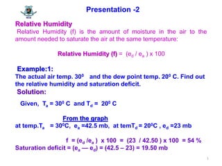
1. 1
Presentation -2
Relative Humidity
Relative Humidity (f) is the amount of moisture in the air to the
amount needed to saturate the air at the same temperature:
Relative Humidity (f) = (ed / ea ) x 100
Example:1:
The actual air temp. 300 and the dew point temp. 200 C. Find out
the relative humidity and saturation deficit.
Solution:
Given, Ta = 300 C and Td = 200 C
From the graph
at temp.Ta = 300C, ea =42.5 mb, at temTd = 200C , ed =23 mb
f = (ed /ea ) x 100 = (23 / 42.50 ) x 100 = 54 %
Saturation deficit = (ea — ed) = (42.5 – 23) = 19.50 mb
3. 3
1.8.5 Absolute Humidity
Absolute Humidity (ρw ) : The ratio between the mass of water vapor
per unit volume of air at a given temperature and is equivalent to the
vapor density is called absolute humidity.
Thus if a volume V (m3)of air contains mw (g) of water vapor ,
then
Absolute Humidity (ρw ) = {Mass of water vapor (g) }/{Volume of air (m3)}
ρw = mw / V (gm-3)
Presentation-2(contd.)
4. 4
Presentation-2(contd.)
Specific Humidity
Specific Humidity (q): The ratio of the mass of water vapor
(mwg) to the mass of moist air (in kg) in a given volume is
called specific humidity.
This is the same as relating the absolute humidity (gm-3) to the
density of the same volume of unsaturated air (ρ in kg m-3):
q = mw (g)/ ( mw + md ) (kg) = ρw /ρ (g kg-1)
where,
md is the mass of the dry air in kg
mw is the mass of water vapor in g
5. 5
Precipitable water
Precipitable water: The total amount of water vapor in a
column of air expressed as the depth of liquid water in
millimeters over the base area of the column Figure 1. The
precipitable water gives an estimate of maximum possible
rainfall
In a column of unit cross sectional area , a small
thickness, dz, of moist air contains a mass of water
given by :
d mw = ρw x dz
Presentation-2(contd.)
6. 6
Thus , in a column of air from heights
z1 to z2 corresponds pressure p1 to p2
z2
the total mass of water mw = ∫ ρw dz
z1
Also, dp = - ρg dz
dz = - dp / pg
Thus : p2
the total mass of water , mw = ∫ ρw dz
p1
z1
z2P2
p1
Columnofair(mw)
Presentation-2(contd.)
Figure-1
7. 7
Thus : p2
the total mass of water , mw = ∫ ρw dz
p1
p2 p2
mw = ∫ ρw / ρg (- dρ) = - ∫ (ρw /ρg) dp
p1 p1
p1
= (1/g) ∫(q )dp
p2
Converting mass water (mw) into equivalent depth over a unit
cross sectional area, the precipitable water is given by
P1
W (mm) = (0.1/ g) ∫ q dp
p2
where, p is in mb, q = ρw /ρg in g kg -1 and g = 9.81 ms-2
Presentation-2(contd.)
8. 8
In practice it is not possible to integrate until q is not
known as function of p.
However a value of W is obtained by summing up the
contribution for a sequence of layers in the troposphere
from a series of measurement of the specific humidity (q)
of air at different heights and using the average specific
humidity q over each layer with the appropriate pressure
difference:
p1
W(mm) = (0.1/ g) ∑ q ∆p
p2
Presentation-2(contd.)
9. 9
Radiosonde
Radiosonde is a battery-powered telemetry instrument carried into the
atmosphere usually by a weather balloon that measures various
atmospheric parameters and transmits them by radio to a ground receiver.
Modern radiosondes measure or calculate the following variables: altitude,
pressure, temperature, relative humidity, wind (both wind speed and wind
direction), cosmic ray (cosmic rays are high–energy radiation, mainly
originating outside the Solar System and even from distant galaxies.
Upon impact with the Earth’s atmosphere, cosmic rays can produce
showers of secondary particles that sometimes reach the surface)
readings at high altitude and geographical position (latitude/ longitude).
Radiosondes measuring ozone concentration are known as
ozonesondes
10. 10
Presentation-2(contd.)
Example:1-2 The following aerological observations shown
in Data table below were taken from a radiosonde ascent. If
60% of the precipitable water is produced from the air up to the
600 mb level to form precipitation at ground level, what would
be the depth of the rainfall?
Pressure(p)-
( mb)
1006 920 800 740 700 660 600 500 400
Specific
humidity
(gkg-1)
14.0 13.4 10.2 9.4 7.2 6.6 5.6 4.0 1.8
Data Table
11. 11
Presentation-2(contd.)
We know total precipitable water, W
p1
W(mm) = (0.1 /g) ∑ q ∆p
p2
Solution
Given
Pressure and specific humidity Data in the table.
Precibitable water is produced from the air up to the 600 mb
level to form precipitation at ground level,
To be calculated depth of rainfall if 60% of the precipitable
water forms rainfall.
Pressure calculation at different height
∆p1 = 1006-920 = 86 mb
∆p2 = 920-800 = 120 mb
and so on.......
13. 13
Presentation-2(contd.)
Total q (mean) * ∆p
p1
∑ q ∆p = 1178.2+1416.0+588.0 + 332.0 + 276.0 + 366.0
p2
= 4156.2
Total the precipitable water up to 600 mb level
p1
W(mm) = (0.1/ g) ∑ q (mean)* ∆p = 4156.2 * 0.1) / g = 42.36 mm
p2
As given 60% of the precipitable water only will produce
rainfall, therefore, depth of rainfall will be = 42.36 mm * 60%
= 25.4 mm .
14. 14
Precipitation
All forms of water that reaches the earth from the atmosphere.
The characteristics for the formation of precipitation are :
1. the atmosphere must have moisture
2. there must be sufficient nuclei present to aid condensation
3. weather conditions must be favorable for condensation of
water vapor to take place.
4. the products of condensation must reach the earth .
Presentation 2 (contd.)
1.rainfall
2. snowfall
5.hail
6.sleet
3.drizzle
4.glaze
The usual forms of precipitation
15. 15
Presentation-2(contd.)
1.Rainfall:
The precipitation in the form of water drops of sizes larger
than 0.50 mm per unit time is rainfall .
The maximum size of rain drop is about 6 mm. On the
basis of its intensity rainfall is classified as the following:
Sl.No Type Intensity
1 Light rain trace to 2.50 mm/hr
2 Moderate rain 2.5 mm /hr to 7.5 mm/hr
3 Heavy rain > 7.5 mm/hr
16. 16
2. Snow: Another form of precipitation
consists of ice crystals which usually
combine to form flake (small piece of
something). When new, snow has an
initial density varying from 0.06 to 0.15
g/cm3 and it is usual to assume an
average density of 0.1 g/cm3
3. Drizzle
A fine sprinkle of numerous water
droplets of size has less than 0.50
mm and intensity less than 1 mm /hr
is known as drizzle. The rain drops
are so small that they float in the air.
Presentation-2(contd.)
17. 17
Presentation-2(contd.)
4. Glaze
When rain or drizzle
comes in contact with cold
ground at around 00 C, the
water drops freeze to form
an ice coating called glaze
or freezing rain.
5. Sleet
It is frozen rain drops of
transparent grains which form
when rain falls through air at
sub freezing temperature. In
Britain sleet means
precipitation of snow and rain
simultaneously.
6. Hail
It is a showery precipitation in the
form of irregular pellets or lumps
of ice as size more than 6 mm.
Hails occur in violent thunder
storms in which vertical currents
are very strong.
18. 18
Presentation-2(contd.)
WEATHER SYSTEM
Precipitation
The moist air masses cool to form condensation and form
nuclei after that fall on the surface of the earth is called
precipitation.
Types of precipitation
5types
(1) Frontal
(2) Cyclone (4) Convective
(3)Anti Cyclone
(5) Orographic
(i) Tropical
(ii)Extra tropical
19. 19
(1) Frontal : A front is the interface between two distinct
air masses. Under certain favorable conditions when an air
mass and cold air mass meet, the warmer air mass is lifted
over the colder one with the formation of a front. The
ascending warmer air cools with the consequent formation
of clouds and precipitation.
(2) Cyclone : A cyclone is a large low
pressure region with circular wind motion.
Cyclone is of two types:
Presentation-2(contd.)
20. 20
(ii) Extra tropical cyclones:
These cyclones are formed in
locations outside the tropical
zone. They posses a strong
counter clockwise wind
circulation in the northern
hemisphere. The magnitude of
the precipitation and wind
velocities are relatively lower
than those of tropical cyclone.
(i) Tropical cyclone – Tropical
cyclone is a wind system with
an intensely strong depression
with MSL pressure sometimes
below 915 mbars. A tropical
cyclone is also called cyclone in
India and Bangladesh, hurricane
in USA and typhoon in South
Asia.
Types of cyclone- Two types
Presentation-2(contd.)
21. 21
(3) Anti cyclone: These are
regions of high pressure,
usually of large areal extent.
The weather is usually calm
at the centre. Anticyclones
cause clockwise wind
circulations in the northern
hemisphere. Winds are of
moderate
(5) Orographic precipitation : The moist air mass
may get lifted up to higher due to the presence of
mountain barriers and consequently undergo
cooling, condensation and precipitation. Such a
precipitation is called orographic precipitation.
4.Convective precipitation: It is
caused by the rising of warmer,
lighter air in colder, denser
surroundings. The difference in
temperature may result from
unequal heating at the surface,
unequal cooling at the top of the
air layer , or mechanical lifting
when the air is forced to pass
over denser, colder air mass or
over a mountain barrier.
Presentation-2(contd.)
22. 22
Measurement of precipitation
Precipitation is expressed in terms of the depth to which
rainfall water would stand on an area if all the rain were
collected on it. Thus 1 cm of rainfall over a catchment area
of 1 km2 represents a volume of water equal to 104 m3.
The precipitation is collected and measured in a rain gauge
– Such as
(1) Pluviometer
(2) Ombrometer
(3) hyetometer
Presentation-2(contd.)
23. 23
Presentation-2(contd.)
Rain gauge
A rain gauge consists of a cylindrical- vessel assembly kept
in the open to collect rain. The rainfall catch of the rain gauge
is affected by its exposure conditions.
The important conditions for setting a rain gauge
are :
(i) the ground must be level and in the open and the
instrument must present a horizontal catch surface
(ii) the gauge must be set as near the ground as
possible to reduce wind effects but it must be a
sufficiently high to prevent splashing, flooding etc.
24. 24
Presentation-2(contd.)
Rain gauge
Obstroucle
h
30m or 2* h
which one is greater
5.5 m * 5.5 m
(iii) the instrument must be surrounded by an open faced
area of at least 5.5m x 5.5 m.
(iv) No object should be nearest to the instrument than 30 m
or twice the height of the obstruction.
25. 25
Rain gauge classification:
Broadly Rain gauge is of two types:
(a) Non recording rain gauges
(b) Recording Rain gauges
(a) Non recording Rain gauge:
Extensively used is ‘ Symons’ gauge :
It consists of a circular collecting area of 12.70 cm(5 inch)
diameter connected to a funnel. The rim of the collector is set
in a horizontal plane at a height of 30.50 cm above ground
level. The funnel discharges the rainfall catch into a receiving
vessel. The funnel and receiving vessel are housed in a
metallic container.
Presentation-2(contd.)
26. 26
Concrete block
600 mm * 600mm * 600 mm
30.5cm
12.70 cm 2.54 cm
Funnel
Collecting bottle
Metal outer container
GL
20.3cm
Figure : Non recording rain gauge
The water contained in the recording vessel is measured by a
suitable graduated measuring glass with a n accuracy up to
0.10mm. The rainfall is measured every day at 8.30 am and is
recorded as the rainfall of the day.
Presentation-2(contd.)