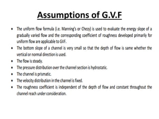
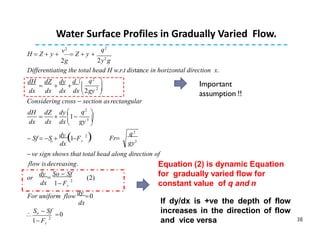
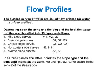
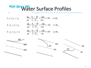
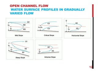
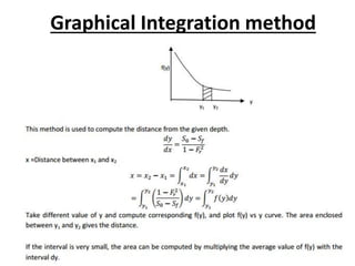
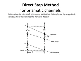
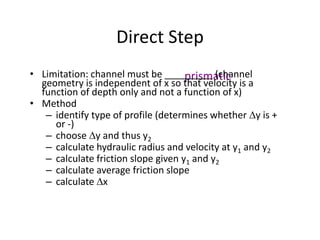
The document summarizes concepts related to gradually varied flow in open channels. It discusses: 1. The assumptions and equations used in gradually varied flow analysis, including the energy equation. 2. The different types of water surface profiles that can occur depending on factors like bed slope, including mild slope, steep slope, critical slope, horizontal slope, and adverse slope profiles. 3. Methods for computing gradually varied flow profiles, including graphical integration, direct step method for prismatic channels, and standard step method for natural channels.

1. Chapter 7
Non uniform Gradually varied
flow(GVF)
1
Hydraulics
Er. Binu Karki
Lecturer

4. Occurance of G.V.L

5. Assumptions of G.V.F

6. Energy Equation for Gradually Varied Flow.
Z1
V2
1
2g
Datu
m
S
o
y1
Z2
V2
2
2g
y2
HG
L
E
L
Water
Level
VV
 hl
2
2
2 g
 Z  y 2 2
2
1
2 g
Z 1  y 1 
Theoretical
EL
Sw
hL
∆
X
∆
L
S
Remember: Both sections are subject to atmospheric
pressure
6

7. Energy Equation for Gradually Varied Flow.
7
V
ohL
Sf So

X LL
Sf 
(1)
, So 
2g2g
L 
E1  E2
Now
E1  E2  So L SfL
Z1  Z2  Z1  Z2 
 Z1  Z2  hL
2
2
2
2
y 
V1
 y 1
for   6
Where L  length of water surface profile
An approximate analysis of gradually varied, non uniform flow can
be achieved by considering a length of stream consisting of a
number of successive reaches, in each of which uniform occurs.
Greater accuracy results from smaller depth variation in each reach.
V
2g2g
Z2  hL
2
2
2
2
y 
V1
 y 1Z1 +

8. Energy Equation for Gradually Varied Flow.
8
m
m
mm
R4/3
V2
n2
n
V
S 

1
R2 /3
S1/ 2
The Manning's formula (or Chezy’s formula) is applied to average
conditions in each reach to provide an estimate of the value of S for that
reach as follows;
2
R
V
m
m
2

R1  R2

V1 V2
In practical, depth range of the interest is divided into small increments,
usually equal, which define the reaches whose lengths can be found by
equation (1)

9. Water Surface Profiles in Gradually Varied
Flow.
Z1
V2
1
2g
Datu
m
S
o
y1
Z2
V2
2
2g
y2
HG
L
E
L
Water
Level
V
HeadTotal
2 g
2
 Z  y 
Theoretical
EL
Sw
h
9
L
∆
X
∆
L

10. Water Surface Profiles in Gradually Varied Flow.
(2)
2
2
2
2

2
3 


  1



 
  
r
r
o r
1 F

So  Sf
0
For uniform flow
dy
0
dx
1 Fdx
dy

So  Sf
or
flow isdecreasing.
ve sign shows that total head along direction of
q
gy3
dx
 Sf  S 
dy
1F
q2
dx dx dx  gy
dH dZ dy 
Considering cross  section asrectangular
q2
dx dx dx dx 2gy
dH dZ dy d 
Differentiating the total head H w.r.t distance in horizontal direction x.
2y2
g
q2
v2
H  Z  y   Z  y 
2g
Fr
Equation (2) is dynamic Equation
for gradually varied flow for
constant value of q and n
If dy/dx is +ve the depth of flow
increases in the direction of flow
and vice versa 38
Important
assumption !!

11. Water Surface Profiles in Gradually Varied Flow.
y10/3
n2
q2
S 
orq 
1
y5/3
S1/ 2
n
orV 
1
y2 / 3
S1/ 2
n
For a wide rectangular channel
R  y dx 1 Fr2
dy

So  Sf
c Consequently, for constant q and n,
when y>yo, S<So, and the numerator
is +ve.
c Conversely, when y<yo, S>So, and
the numerator is –ve.
c To investigate the denominator we
observe that,
c if F=1,dy/dx=infinity;
c if F>1,the denominator is -ve; and
c if F<1,the denominator is +ve.
39

12. Types of Bed Slopes
12
 Mild Slope (M)
yo > yc
So < Sc
 Critical Slope (C)
yo = yc
So = Sc
 Steep Slope (S)
yo < yc
So > Sc
So1<S
c
yo1
yc
yo2
Break
So2>Sc
y = normal depth of flowo
yc= critical depth
So= channel bed slope
Sc=critical channel bed slope

13. Occurrence of Critical Depth
13
 Change in Bed Slope
 Sub-critical to Super-Critical
 Control Section
 Super-Critical to Sub-Critical
 Hydraulics Jump
Control Section
So1<S
c
So2>S
c
yo1
yo2
y
c
Break where
Slope
changes
Dropdown Curve
So1>S
c
yo1
yo2
y
c
Hydraulic Jump
So2<S
c

14. Flow Profiles
The surface curves of water are called flow profiles (or water
surface profiles).
Depending upon the zone and the slope of the bed, the water
profiles are classified into 13 types as follows:
1. Mild slope curves M1, M2, M3
2. Steep slope curves S1, S2, S3
3. Critical slope curves C1, C2, C3
4. Horizontal slope curves H2, H3
5. Averse slope curves A2, A3
In all these curves, the letter indicates the slope type and the
subscript indicates the zone. For example S2 curve occurs in the
zone 2 of the steep slope

15. Classification of Surface Profiles
15

17. Water Surface Profiles
17
Mild Slope (M)
1
2
3
1: y  yo  yc
dy

So  Sf

Ve
 Ve  M
dx 1 Fr 2 Ve
2 : yo  y  yc
dy

So  Sf

Ve
 Ve  M
dx 1 Fr 2 Ve
3 : yo  yc  y
dy

So  Sf

Ve
 Ve  M
dx 1 Fr 2 Ve

18. Water Surface Profiles
Steep Slope (S)
1
2
3
1: y  yc  yo
dy

So  Sf

Ve
 Ve  S
dx 1 Fr 2 Ve
2 : yc  y  yo
dy

So  Sf

Ve
 Ve  S
dx 1 Fr 2 Ve
3 : yc  yo  y
dy

So  Sf

Ve
 Ve  S
dx 1 Fr 2 Ve

19. Water Surface Profiles
Critical (C)
19
1
3
1: y  yo  yc
dy

So  Sf

Ve
 Ve  C
dx 1 Fr 2 Ve
2 : yo  yc  y
dy

So  Sf

Ve
 Ve  C
dx 1 Fr 2 Ve
C2 is not
possible

20. Water Surface Profiles
Horizontal (H)
20
2
3
c
c
o()
o()
1: y  y 
y
dy 
So Sf Ve
 Ve 
H
Ve
2 : y  y  y
dx 1 Fr 2
dy 
So-Sf
dx 1 Fr 2
 Ve
 Ve 
H
Ve
H1 is not possible bcz water has to lower
down

21. Water Surface
Profiles
Adverse (A)
2
3
c
c
o()
o()
1: y  y  y
dy

So  Sf 
Ve
 Ve  A
Ve
2: y  y  y
dx 1 Fr2
dy

So-Sf
dx 1 Fr2

Ve
 Ve  A
Ve
A1 is not possible bcz water has to lower
down

22. OPEN CHANNEL FLOW
WATER SURFACE PROFILES IN GRADUALLY
VARIED FLOW
12

23. COMPUTATION OF G.V.F
1.Graphical Integration method
2.Direct step method
3.Standard step method

24. Graphical Integration method

25. Direct Step Method
for prismatic channels

26. xS
g
V
yxS
g
V
y fo 
22
2
2
2
2
1
1
of SS
g
V
g
V
yy
x



22
2
2
2
1
21
energy equation
solve for x
1
1
y
q
V 
2
2
y
q
V 
2
2
A
Q
V 
1
1
A
Q
V 
rectangular channel prismatic channel

27. prismatic
Direct Step
• Limitation: channel must be _________ (channel
geometry is independent of x so that velocity is a
function of depth only and not a function of x)
• Method
– identify type of profile (determines whether y is +
or -)
– choose y and thus y2
– calculate hydraulic radius and velocity at y1 and y2
– calculate friction slope given y1 and y2
– calculate average friction slope
– calculate x

28. Direct Step Method
of SS
g
V
g
V
yy
x



22
2
2
2
1
21

29. Standard Step
For natural channels
• Given a depth at one location, determine the depth at a
second given location
• Step size (x) must be small enough so that changes in
water depth aren’t very large. Otherwise estimates of
the friction slope and the velocity head are inaccurate
• Can solve in upstream or downstream direction
– Usually solved upstream for subcritical
– Usually solved downstream for supercritical
• Find a depth that satisfies the energy equation
xS
g
V
yxS
g
V
y fo 
22
2
2
2
2
1
1