Chapter summary and solutions to end-of-chapter exercises for "Data Visualization: Principles and Practice" book by Alexandru C. Telea Chapter provides an overview of a number of methods for visualizing tensor data. It explains principal component analysis as a technique used to process a tensor matrix and extract from it information that can directly be used in its visualization. It forms a fundamental part of many tensor data processing and visualization algorithms. Section 7.4 shows how the results of the principal component analysis can be visualized using the simple color-mapping techniques. Next parts of the chapter explain how same data can be visualized using tensor glyphs, and streamline-like visualization techniques. In contrast to Slicer, which is a more general framework for analyzing and visualizing 3D slice-based data volumes, the Diffusion Toolkit focuses on DT-MRI datasets, and thus offers more extensive and easier to use options for fiber tracking.

1. DS-620 Data Visualization
Chapter 7 Summary.
Valerii Klymchuk
August 19, 2015
0. EXERCISE 0
7 Tensor Visualization
Tensor data encode some spatial property that varies as a function of position and direction, such as curvature
of a three-dimensional surface at a given point and direction. Every point in a tensor dataset carries a 3 × 3
matrix. Material properties such as stress and strain in 3D volumes, are described by stress tensors. Diffusion
of water in tissues can be described by a 3 × 3 diffusion tensor matrix. In human brain diffusion is stronger
in the direction of the neural fibers and weaker across fibers. By measuring the diffusion, we can get insight
into complex structure of neural fibers in the human brain. The measurement of the diffusion of water in
living tissues is done by a set of techniques known as diffusion tensor magnetic resonance imaging
(DT-MRI). The process that constructs visualizations of the anatomical structures of interest starting from
the measured diffusion data is known as diffusion tensor imaging (DTI).
Intrinsic structure of the tensor data can be exploited by computations called principal component
analysis.
7.1 Principal Component Analysis
We have shown that we can compute the normal curvature at some point x0 in some direction s in the tangent
plane as the second derivative ∂2
f/∂s2
of f using the two-by-two Hessian matrix of partial derivatives of f.
Minimal and maximal values of the curvature at a given point are invariant to the choice of the (direction)
local coordinate system since they depend only on the surface shape at a given point.
The direction in the tangent plane for which the normal curvature has extremal values are the solutions
of the following equation:
Hs = λs.
For 2 × 2 matrices we can solve the equation analytically, obtaining two solutions λ1 and s1 and λ2 and
s2, respectively:
The surface has minimal curvature in the direction s1 and maximal curvature in the direction s2. Along
all directions in the tangent plane orthogonal to the surface normal, the curvature takes values between the
minimal and maximal ones.
The solutions si are called the principal directions, or eigenvectors of the tensor H, and values λi
are called eigenvalues. For n×n symmetric matrix, the principal directions are perpendicular to each other
and form directions in which the quantity reaches extremal values.
In the case of a 3D surface given by an implicit function f(x, y, z) = 0 in global coordinates, we have a
3 × 3 Hessian matrix of partial derivatives, which has 3 eigenvalues and three eigenvectors that we compute
by solving equation. A good method is the Jacobi iteration method, which solves Equation numerically for
arbitrary-size n × n real symmetric matrices.
If we order the eigenvalues in decreasing order λ1 > λ2 > λ3, the corresponding eigenvectors e1, e2 and
e3, also called the major, medium, and minor eigenvalues , that have following meaning. In case of
1

2. curvature tensor, e1, e2 are tangent to the given surface and give the directions of maximal and minimal
normal curvature on the surface, and e3 is equal to the surface normal.
7.2 Visualizing Components
The simples way to visualize a tensor dataset is to treat it as a set of scalar datasets. Given a 3 × 3 tensor
matrix we can consider each of its nine components hij as a separate scalar field.
Each component of the tensor matrix is visualized using grayscale colormap that maps scalar value to
luminance. Note, that due to the symmetry of the tensor matrix, there are only 6 different images in
the visualization (h12 = h21, h13 = h31, h23 = h32). In general, the tensor matrix components encode the
second-order partial derivatives of our tensor-encoded quantity with respect to the global coordinate system.
7.3 Visualizing Scalar PCA Information
A better alternative to visualizing the tensor matrix components is to focus on data derived from these
components that has a more intuitive physical significance.
Diffusivity. The mean of the measured diffusion over all directions at that point is measures as the
average of the diagonal entries: 1
3 (h11 + h22 + h33).
Anisotropy. Recall, that eigenvalues give the values of the extremal variations in directions of eigen-
vectors (extremal variations). In case of diffusion data, the eigenvalues can be used to describe the degree
of anisotropy of the tissue at a point (different diffusivities in different directions around the point).
A set of metrics proposed by Westin, estimates the certainties cl, cp, and cs that a tensor has a linear,
planar, or spherical shape, respectively. If the tensor’s eigenvalues are λ1 ≥ λ2 ≥ λ3, the respective certainties
are
cl =
λ1 − λ2
λ1 + λ2 + λ3
cp =
2(λ2 − λ3)
λ1 + λ2 + λ3
cs =
3λ3
λ1 + λ2 + λ3
.
A simple way to use the anisotropy metrics proposed previously is to directly visualize the linear certainty
cl scalar signal.
Another frequently used measure for the anisotropy is the fractional anisotropy, which is defined as
FA =
3
2
3
i=1(λi − µ)2
λ2
1 + λ2
2 + λ2
3
,
where µ = 1
3 (λ1 + λ2 + λ3) is the mean diffusivity.
A related measure is the relative anisotropy, defined as
RA =
3
2
3
i=1(λi − µ)2
λ1 + λ2 + λ3
.
Methods in this section reduce the visualization of a tensor field to that of one or more scalar quantities.
These can be examined using any of the scalar visualization methods such as color plots, slice planes, and
isosurfaces.
7.4 Visualizing Vector PCA Information
Let’s say, we are interested only in the direction of maximal variation of our tensor-encoded quantity. For
this we can visualize the major eigenvector field using any of the vector visualization methods in Chapter 6.
Vectors can be uniformly seeded at all points where the accuracy of the diffusion measurements is above a
2

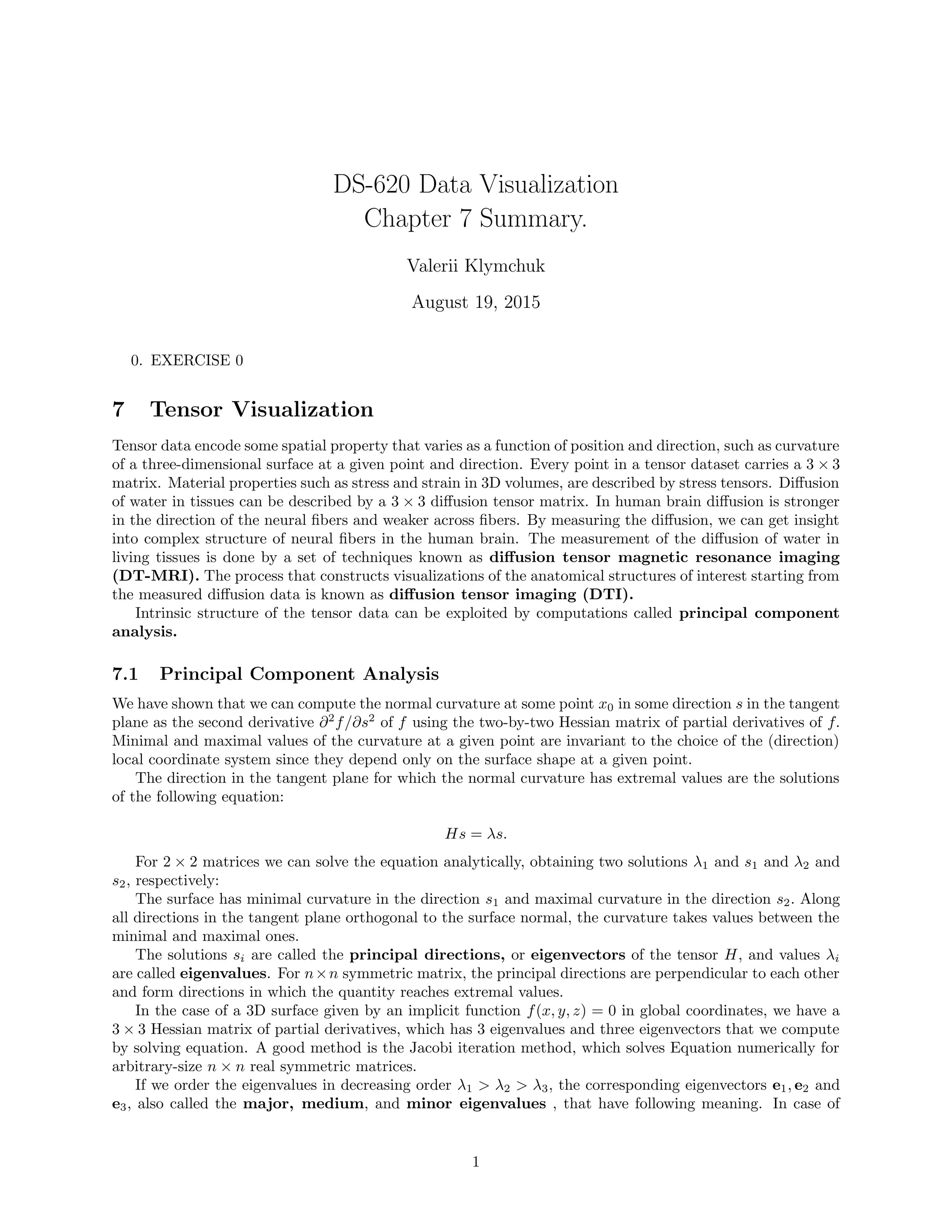
3. certain confidence level. The hue of the vector coloring can indicate their direction, by using the following
colormap:
R = |e1 · x|
G = |e1 · y|
B = |e1 · z|
.
The luminance can indicate the measurement confidence level. A relatively popular technique in this
class is to simply color map the major eigenvector direction.
Visualizing a single eigenvector or eigenvalue at a time may not be enough. In many cases the ratios of
eigenvalues, rather than their absolute values, are of interest.
7.5 Tensor Glyphs
We sample the dataset domain with a number of representative sample points. For each sample point, we
construct a tensor glyph that encodes the eigenvalues and eigenvectors of the tensor at that point. For
a 2 × 2 tensor dataset we construct a 2D ellipse whose half axes are oriented in the directions of the two
eigenvectors and scaled by the absolute values of the eigenvalues. For a 3 × 3 tensor we construct a 3D
ellipsoid in a similar manner.
Besides ellipsoids, several other shapes can be used: like parallelepipeds (cuboids), or cylinders instead
of ellipsoids. Smooth glyph shapes like those provided by the ellipsoids provide a less-distracting picture,
than shapes with sharp edges, such as the cuboids and cylinders.
Superquadric shapes are parameterized as functions of the planar and linear certainty metrics cl and cp,
respectively.
Another tensor glyph used is an axes system, formed by three vector glyphs that separately encode
the three eigenvectors scaled by their corresponding eigenvalues. This method is easier to interpret for 2D
datasets, however in 3D they create too much confusion due to spatial overlap.
Eigenvalues can have a large range, so directly scaling the tensor ellipsoids by their values can easily lead
to overlapping and (or) very thin or very flat glyphs. We can solve this problem as we did for vector glyphs
by imposing a minimal and maximal glyph size, either by clamping or by using a nonlinear value-to-size
mapping function.
7.6 Fiber Tracking
In case of a DT-MRI tensor dataset, regions of high anisotropy in general, and of high values of the cl
linear certainty metric in particular, correspond to neural fibers aligned with the major eigenvector e1. If
we want to visualize the location and direction of such fibers, it is natural to think of tracking the direction
of this eigenvector over regions of high anisotropy by using the streamline technique. First, a seed region is
identified. This is a region where the fibers should intersect, so it can be detected by thresholding one of the
anisotropy metrics presented in section 7.3. Second, streamlines are densely seeded in this region and traced
(integrated) both forward and backward in the major eigenvector field e1 until a desired stop criterion is
reached (minimal value of anisotropy reached, or a maximal distance from other tracked fibers).
After the fibers are tracked, they can be visualized using the stream tubes technique. The constructed
tubes can be colored to show the value of a relevant scalar field, the major eigenvalue, anisotropy metric, or
some other quantity scanned along with the tensor data.
Focus and context. Fiber tracks are most useful when shown in context of the anatomy of the brain
structure being explored.
Fiber clustering. Given two fibers a = a(t) and b = b(t) with t ∈ [0, 1] we first define distance:
d(a, b) =
1
2N
N
i=1
(||a(i/N), b|| + ||b(i/N), a||) ,
as symmetric mean distance of N sample points on a fiber to the (closest points on) other fiber. The
directional similarity of two fibers is defined as the inverse of the distance. Using the distance, the tracked
fibers are next clustered in order of increasing distance, i.e. from the most to the least similar, until the desired
3

4. number of clusters is reached. For this simple bottom-up hierarchical agglomerative technique introduced in
Section 6.7.3 for vector fields can be used.
Tracking challenges. First, tensor data acquired via the current DT-MRI scanning technology contains
in practice considerable noise and has a sampling frequency that misses several fine-scale details. Moreover,
tensors are not directly produced by the scanning device, but obtained via several processing steps, of which
principal component analysis is the last one. All these steps introduce extra inaccuracies in the data, which
have to be accounted for. The PCA estimation of eigenvectors can fail if the tensor matrices are not close to
being symmetric. Even if PCA works, fiber tracking needs a strong distinction between the largest eigenvalue
and the other two ones, in order to robustly determine the fiber direction.
7.7 Illustrative Fiber Rendering
While some approaches are easy to implement, they give “raw” view on the fiber data, which has several
problems:
• Region structure: Fibers are one-dimensional objects. However, to better understand the structure of
the DTI tensor field, we would like to see the linear anisotropy regions with fibers and planar anisotropy
regions rendered as surfaces.
• Simplifications: Densely-seeded datasets can become highly cluttered, so it is hard to discern the global
structure implied by the fibers. A simplified visualization of fibers can be useful in understanding
relative depth of fibers.
• Context: Showing combined visualizations of fibers and tissue density can provide more insight into
the spatial distribution and connectivity patterns implied by fibers.
A set of simple techniques can address the above goals.
Fiber generation. We densely seed the volume and trace fibers using Diffusion Toolkit. Each resulting
fiber is represented as polyline consisting of an ordered set of 3D vertex coordinates.
Alpha blending. One simple step to reduce occlusion and see inside the fiber volume is to use additive
alpha blending (Section 2.5). However, fibers need to be sorted back-to-front as seen from the viewing
angle. One simple way to do this efficiently is to transform all fiber vertices in eye coordinates, i.e., in a
coordinate frame, where the x- and y-axes match the screen x- and y-axes, and $z-%axis is parallel to the
view vector, and next to sort them based on their z value. Sorting has to be executed every time we change
the viewing direction.
Anisotropy simplification. Alpha blending reduces occlusion, but it akts in a global manner. We
however, are specifically interested in regions of high anisotropy. To emphasize such regions we next modulate
the colors of the drawn fiber points by the value of the combined linear and planar anisotropy
ca = cl + cp = 1 − cs =
λ1 + λ2 − 2λ3
λ1 + λ2 + λ3
, where cl, cp,and $c s $are the linear, planar and spherical anisotropy metrics. IF we render fiber points
having ca > 0.2 color-coded by direction, and all other fiber points in gray. The image shows well the fiber
subset which passes through regions of linear and (or) planar anisotropy, i.e., separates interesting from less
interesting fibers. Using anisotropy to cull fiber fragments after tracing is a less aggressive, and offers more
chances for meaningful fiber fragments to exist in the final visualization, without having to be very precise
in the selection of the anisotropy threshold used.
Illustrative rendering.
Here we construct stream tube-like structures around the rendered fibers. However instead of using 3D
space stream tube algorithm, we densely sample all fiber polylines, and render each resulting vertex with
an OpenGL sprite primitive that uses a small 2D texture. The texture encodes the shading profile of a
sphere, i.e., is bright at the middle and dark at the border. Compared to streamtubes, the advantage of this
technique is that it is much simpler to implement, and also much faster, since there is no need to construct
complex 3D tubes, we only render one small 2D texture per fiber vertex.
A second option for illustrative (simplified) rendering of fiber tracks entails using the depth-dependent
halos method presented for vector field streamlines in Section 6.8. Depth dependent halos effectively merge
4

5. dense fiber regions into compact black areas, but separate fibers having different depth by a thin white halo
border. Together with interactive viewpoint manipulation, this helps users in perceiving the relative depths
of different fiber sets.
Fiber bundling. We still cannot easily visualy distinguish regions of linear and planar anisotropy from
each other. WE cannot visually classify dense fiber regions as being (a) either thick tubular fiber bundles or
(b) planar anisotropy regions covered by fibers.
In order to simplify the structure of the fiber set, we apply a clustering algorithm, as follows: Given
a set of fibers, we first estimate a 3D fiber density field ρ : R3
→ R+
, by convolving the positions of
all fiber vertices, or sample points, with a 3D monotonically decaying kernel, such as Gaussian or convex
parabolic function. Next, we advect each sample point upstream in the normalized gradient ρ/|| ρ|| of the
density field, and recompute the density ρ of the new fiber sample points. Iterating this process 10..20 times
effectively shifts the fibers towards their local density maxima. In other words kernel density estimation
creates compact fiber bundles that describe groups of fibers which are locally close to each other.
The bundled fibers occupy much less space, thus allow a better perception of the structure of the brain
connectivity pattern they imply. However effective in reducing spatial occlusion and thereby simplifying
the resulting visualization, fiber bundling suffers from two problems. First, planar anisotropy regions, are
reduced to a few one-dimensional bundles. This conveys wrong impression. Second, bundling effectively
changes the positions of fibers. As such, fiber boundless should be interpreted with great care, since they
have limited geometrical meaning.
To address the first problem, we can modify the fiber bundling algorithm and instead of using an isotropic
spherical kernel to estimate the fiber density, we can use an ellipsoidal kernel, whose axes are originated along
the directions of the eigenvectors of the DTI tensor field, and scaled by the reciprocals of the eigenvalues of
the same field. In linear anisotropy regions, fibers will strongly bundle towards the local density center, but
barely shift in their tangent directions. In planar anisotropy regions, fibers will strongly bundle towards the
implicit fiber-plane, but barely shift across this plane. Additionally, we use the values of cl and cp to render
the above two fiber types differently. For fiber points located in linear anisotropy regions (cl large) we render
point sprites using spherical textures, for planar anisotropy regions we render 2D quads perpendicular to the
direction of the eigenvector corresponding to the smallest eigenvalue, i.e., tangent to the two underlying fiber
plane. So that in linear anisotropy regions we see tube-like structures, in planar regions - planar structures.
7.8 Hyperstreamlines
First, we perform principal component analysis to decompose the tensor field into three eigenvector fields
ei and three corresponding scalar eigenvalue fields λ1 ≥ λ2 ≥ λ3. Next, we construct streamtubes in the
major eigenvector field e1. At each point along such a streamtube, we now wish to visualize the medium and
minor eigenvectors e2 and e3. For this instead of using a circular cross section of constant size and shape,
we now use an elliptic cross section, whose axes are oriented along the directions of the medium and minor
eigenvectors e2 and e3 and scaled by λ2 and λ3, respectively.
The local thickness of the hyperstreamlines gives the absolute values of the tensor eigenvalues, whereas
the ellipse shape indicates their relative values as well as the orientation of the eigenvector frame along a
streamline.
Besides ellipses, other shapes can be used for the cross section. In general, hyperstreamlines provide
better visualizations than tensor glyphs. However, appropriate seed points and hyperstream length must be
chosen to appropriately cover the domain, which can be a delicate process. Moreover, scaling of the cross
sections must be done with care, in order to avoid overly thick hyperstreamlines that cause occlusion or even
self-injection. For this we can use scaling techniques in Section 6.2.
7.9 Conclusion
Tensor data can be visualized by reducing it to one scalar or vector field, which is then depicted by specific
scalar or vector visualization techniques. The scalar or vector fields can be the direct outputs of the PCA
analysis (eigenvalues and eigenvectors) or derived quantities, such as various anisotropy metrics. Alterna-
tively, tensors can be visualized by displaying several of the PCA results combined in the same view, such
as done by the tensor glyphs or hyperstreamlines.
5

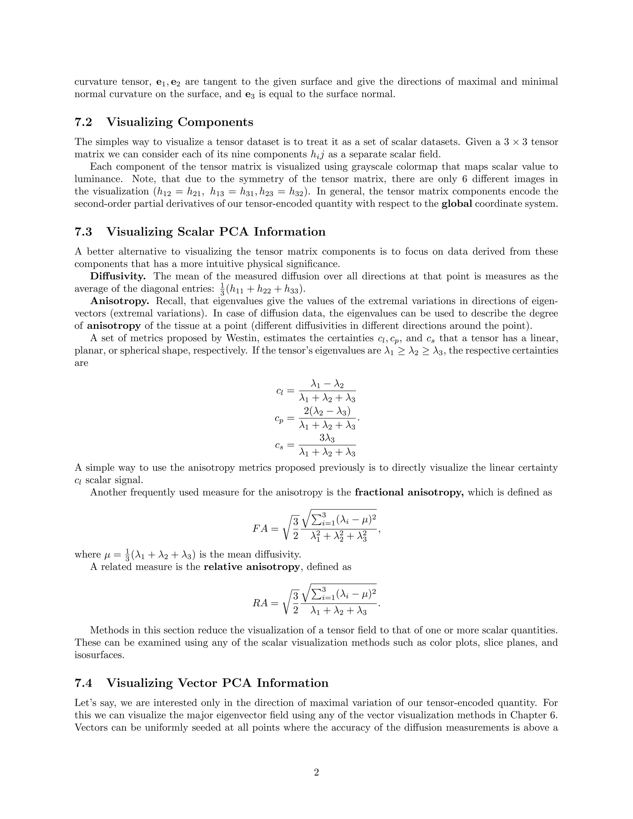
6. What have you learned in this chapter?
Chapter provides an overview of a number of methods for visualizing tensor data. It explains principal
component analysis as a technique used to process a tensor matrix and extract from it information that
can directly be used in its visualization. It forms a fundamental part of many tensor data processing and
visualization algorithms. Section 7.4 shows how the results of the principal component analysis can be
visualized using the simple color-mapping techniques. Next parts of the chapter explain how same data can
be visualized using tensor glyphs, and streamline-like visualization techniques.
In contrast to Slicer, which is a more general framework for analyzing and visualizing 3D slice-based data
volumes, the Diffusion Toolkit focuses on DT-MRI datasets, and thus offers more extensive and easier to use
options for fiber tracking.
What surprised you the most?
• New rendering techniques, such as volume rendering with data-driven opacity transfer functions
are also being developed to better convey complex structures emerging from the tracking process.
• Fiber tracking in DT-MRI datasets is an active area of research.
• Fiber bundling is a promising direction for the generation of simplified structural visualizations of fiber
tracts for DTI fields.
What applications not mentioned in the book you could imagine for the techniques ex-
plained in this chapter?
A hologram 3D glyph can be used in rendering (i.e., semitransparent hyperstreamlines) to mask discon-
tinuities caused by regular tensor glyphs.
Anisotropic bundled visualization of the fiber dataset. We can render the bundled fibers with a translu-
cent sprite texture rendered with alpha blending, while using a kernel of small radius to estimate the
fiiber density ρ. Instead of using an anisotropic sphrical kernel to estimate the fiber density, we use an ellip-
soidal kernel, whose axes are oriented along the directions of the eigenvectors of the DTI tensor field, and
scaled by the reciprocals of the eigenvalues of the same field. In linear anisotropy regions, fibers will strongly
bundle towards the local density center, but barely shift in their tangent directions. In planar anisotropy
regions, fibers will strongly bundle towards the implicit fiber-plane, but barely shift across this plane. We use
the values of cl and cp to render the above two fiber types differently. For fibers in linear anisotropy regions
(cl large), we render point sprites using sphere textures. For fiber points located in planar anisotropy regions
(cp large), we render translucent 2D quads oriented perpendicular to the direction of the eigenvector
corresponding to the smallest eigenvalue.
1. EXERCISE 1
In data visualization, tensor attributes are some of the most challenging data types, due to their high
dimensionality and abstract nature. In Chapter 7 (and also in Section 3.6), we introduced tensor fields by
giving a simple example: the curvature tensor for a 3D surface. Give another example of a tensor field
defined on 2D or 3D domains. For your example
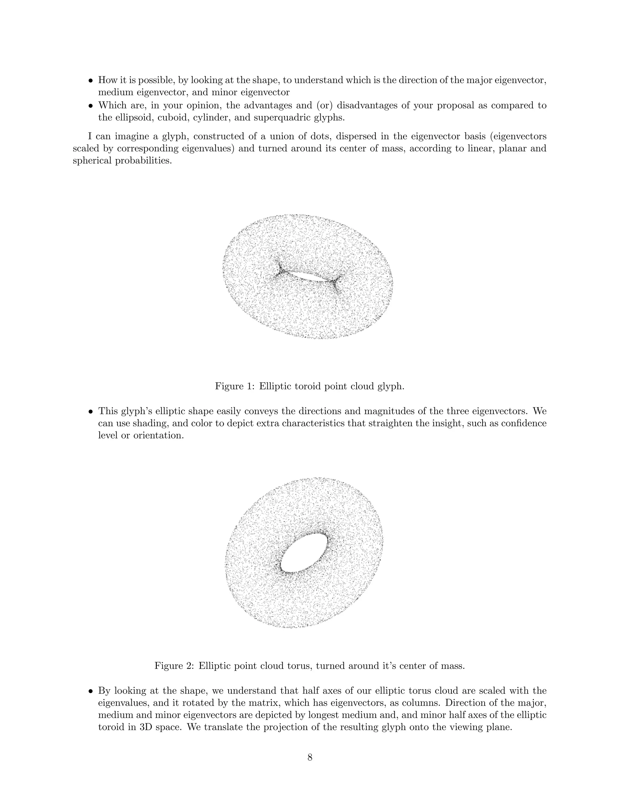
• Explain why the quantity you are defining is a tensor
• Explain how the quantity you are defining varies both as a function of position but also of direction
• Explain what are the intuitive meanings of the minimal, respective maximal, values of your quantity
in the directions of the respective eigenvectors of your tensor field.
• Stress on a material, such as a construction beam in a bridge can be an example of tensor field. Stress
is a tensor because it describes things happening in two directions simultaneously.
Another example is the Cauchy stress tensor T, which takes a direction v as input and produces the
stress T(v) on the surface normal to this vector for output:
σ = [Te1
, Te2
, Te3
] =


σ11 σ12 σ13
σ21 σ22 σ23
σ32 σ32 σ33

 ,
6

7. whose columns are the stresses (forces per unit area) acting on the e1, e2, and e3 faces of the cube.
Other examples of tensors include the diffusion of water in tissues, strain tensor, the conductivity tensor,
and the inertia tensor. Moment of inertia is a tensor too because it involves two directions: the axis of
rotation, and the position of the center of mass.
• quantity describing water diffusivity varies as a function of position (coordinates of the point) and
direction of measurement.
• minimal and maximal values of this quantities are achieved in directions of corresponding eigenvalues:
e1, e2 which are tangent to the given surface and give the directions of maximal and minimal TENSOR
VALUE on the surface, and e3 is equal to the surface normal.
2. EXERCISE 2
Consider a 2-by-2 symmetric matrix A with real-valued entries, such as the Hessian matrix of partial
derivatives of some function of two variables. Now, consider the two eigenvectors x and y of the matrix A,
and their two corresponding eigenvalues λ and µ. We next assume that these eigenvalues are different. Prove
that the two eigenvectors x and y are orthogonal.
Hints: There are several ways to prove this. One way is to use that the matrix is symmetric, hence
A = AT
. Next, use the algebraic identity < Ax, y >=< x, AT
y >, where < a, b > denotes the dot product
of two vectors a and b. To prove that x is orthogonal to y, prove that < x, y >= 0. Based on definition of
eigenvectors and eigenvalues: Ax = λx, Ay = µy.
Let us multiply both sides of the first equation by y and both sides of the second equation by x, so we
get: Axy = λxy, Ayx = µyx. Substituting one from another yilds: Axy − Ayx = λxy − µyx, which means
(λ − µ)xy = 0.
In the equation above λ = µ, which means that xy = 0, there fore vectors x and y are orthogonal.
3. EXERCISE 3
One basic solution for visualizing eigenvectors of a 3-by-3 tensor, such as the one generated from a
diffusion-tensor MRI scan, is to color-code its (major) eigenvector using a directional colormap. Figure 7.6
(also shown below) shows such a colormap, where we modulate the basic color components R, G, and B to
indicate the orientation of the eigenvector with respect to the x, y, and z axes respectively. For the same
task of directional color-coding of a tensor field, imagine a different colormap, which, in your opinion, may
be more intuitive than the red-green-blue colormap proposed here.
Vector color coding is easier to understand in HSV system.
The hue value H we calculate as H = arctg(|e1·z|
|e1·x| , to encode the direction of e1 eigen vector in x × z
view plane.
Saturation S = 1 |e1 · y| of the vector coloring can encode its orientation along y axis orthogonal to
the view plane. We can use additive alpha blending in which fibers need to be sorted back-to-front as
seen from the viewing angle. One simple way to do this efficiently is to transform all fiber vertices in eye
coordinates, i.e., in a coordinate frame, where the x− and z−axes match the screen x and y axes, and y
axis is parallel to the view vector, and next to sort them based on their y value. Sorting has to be executed
every time we change the viewing direction. High values of S will correspond to low values of |e1 · y|, which
will result in vectors oriented along y axis depicted in shades of white.
The luminance V indicates the measurement confidence level. So that bright vectors indicate high
confidence measurement levels, whereas dark vectors indicate low confidence level.
4. EXERCISE 4
Tensor glyphs are a generalization of vector glyphs which attempt to convey three vectors (the eigenvectors
of the tensor-field to be explored) at a given point over its domain. In Section 7.5 (Figure 7.8, also shown
below), four kinds of tensor glyphs are proposed: ellipsoids, cuboids, cylinders, and superquadrics. Propose
a different kind of tensor glyph. Sketch the glyph. For your proposed glyph, explain:
• How the glyph’s properties (shape, shading, color) convey the directions and magnitudes of the three
eigenvectors
7

8. • How it is possible, by looking at the shape, to understand which is the direction of the major eigenvector,
medium eigenvector, and minor eigenvector
• Which are, in your opinion, the advantages and (or) disadvantages of your proposal as compared to
the ellipsoid, cuboid, cylinder, and superquadric glyphs.
I can imagine a glyph, constructed of a union of dots, dispersed in the eigenvector basis (eigenvectors
scaled by corresponding eigenvalues) and turned around its center of mass, according to linear, planar and
spherical probabilities.
Figure 1: Elliptic toroid point cloud glyph.
• This glyph’s elliptic shape easily conveys the directions and magnitudes of the three eigenvectors. We
can use shading, and color to depict extra characteristics that straighten the insight, such as confidence
level or orientation.
Figure 2: Elliptic point cloud torus, turned around it’s center of mass.
• By looking at the shape, we understand that half axes of our elliptic torus cloud are scaled with the
eigenvalues, and it rotated by the matrix, which has eigenvectors, as columns. Direction of the major,
medium and minor eigenvectors are depicted by longest medium and, and minor half axes of the elliptic
toroid in 3D space. We translate the projection of the resulting glyph onto the viewing plane.
8

9. The advantages are:
• Smooth elliptic shape provides a less distracting picture, and creates less discontinuities, than shapes
with sharp edges, such as the cuboids and cylinders.
• 2D projection of a point cloud will better convey a non-ambiguous 3D orientation for eigenvalues
corresponding to equal eigenvalues, when viewed from certain angles, compared to a regular ellipsoid
glyph.
• overlapping clouds, perhaps, will result in more dense (more saturated, brighter and more visible)
areas, which only straighten our visual insight (they are predicted by data not from one, but from
multiple sample points), instead of creating occlusion and clutter.
5. EXERCISE 5
One way to visualize a symmetric 3D tensor field is to reduce it, by principal component analysis (PCA), to
a set of three eigenvectors (v1, v2, v3), whose corresponding lengths are given by three eigenvalues (λ1, λ2, λ3).
Such eigenvectors can be visualized, among other methods, by using vector glyphs. In this context, answer
the two questions below:
• If we use vector glyphs, and since we have three eigenvectors, and all of them encode relevant informa-
tion for the tensor field, why do we usually choose to visualize just the major-eigenvector field, rather
than drawing a single image containing vector glyphs?
• Oriented glyphs such as arrows are typically preferred against unoriented ones (e.g. lines) when vi-
sualizing vector fields. Why do not we use such oriented glyphs, but prefer unoriented glyphs, when
visualizing eigenvector fields?
Answers:
• We truly can use another tensor glyph in practice, called axis system, formed by three vector glyphs
that separately encode the three eigenvectors scaled by their corresponding eigenvalues. However, for
3D datasets they create too much confusion due to the 3D spatial overlap, whereas the rounded convex
ellipsoid shapes tend to be more distinguishable even with small amount of overlap. Also, we often are
interested only in the direction of change, which is always determined by the largest eigenvalue.
• Eigenvectors have an unoriented nature. A tensor is independent of any chosen frame of reference. In
general, any scalar function f(λ1, λ2, λ3) that only depends on the eigenvalues again is an invariant.
As a consequence, also every scalar function of invariants is an invariant itself. Eigenvectors have no
magnitude and no orientation (are bidirectional).
We use the term direction space for the feature space that consists of directions.
The full direction information is represented as a triple of points. Because eigenvectors are normalized,
no additional scaling is needed and all points lie on the surface of the unit sphere. In general, we are only
interested in a single direction or in two selected directions. For a single direction, the direction space is a
2D feature space with a spherical basis. Due to the unoriented nature of the eigenvectors, the space further
reduces to a hemisphere.
Symmetric tensors are separated into shape and orientation. Here, shape refers to the eigenvalues and
orientation to the eigenvectors. Symmetric tensors can be represented as diagonal matrices. The basis for
such a representation is given by the eigenvectors corresponding to the diagonal matrix. For symmetric ten-
sors, the eigenvalues are all real, and the eigenvectors constitute an orthonormal basis. The diagonalization
generally is computed numerically via singular value decomposition (SVD) or principal component analysis
(PCA).
6. EXERCISE 6
Consider a smooth 2D scalar field f(x, y), and its gradient f, which is a 2D vector field. Consider now
that we are densely seeding the domain of f and trace streamlines in f, upstream and downstream. Where
9

10. do such streamlines meet? Can you give an analytic definition of these meeting points in terms of values of
the scalar field f?
Hints: Consider the direction in which the gradient of a scalar field points.
They can meet in critical points, where quantity f reaches its extremal values: sinks downstream, and
sources upstream, where || f|| = 0 and values of f are close to maxima or minima.
7. EXERCISE 7
Consider that we have a (dense) point cloud P = {pi} of N 3D points, which are the samples of a 3D
smooth and non-intersecting surface. Many methods exist for the reconstruction of a meshed surface from
such an unorganized point cloud. However, several such methods require to know the orientation of the
surface normal ni at each sample point pi. Describe in detail a method to compute this normal orientation
based on principal component analysis applied to P.
There are two possibilities:
• Obtain the underlying surface from the acquired point cloud by using surface meshing techniques, and
then computing the surface normals from the mesh by averaging;
• Infer the surface normals from the point cloud dataset directly.
The problem of determining the normal to a point on the surface is approximated by the problem of
estimating the normal of a plane tangent to the surface, which in turn becomes a least-square plane fitting
estimation problem:
• Collect some nearest neighbors of pi, for instance 12;
• Fit a plane to pi and its 12 neighbors;
• Use the normal of this plane as the estimated normal for pi.
Surface normal at a point can be estimated from the surrounding point neighborhood support of the point
(also called k -neighborhood). The solution for estimating the surface normal can be reduced to Principal
Component Analysis of a covariance matrix created from the nearest neighbors of the query point. More
specifically, for each point pi, we assemble the covariance matrix C as follows:
C =
1
3
k
i=1
(pi − p) · (pi − p)T
, C · sj = λj · sj, j ∈ 1, 2, 3,
where k = 12 is the number of point neighbors considered in the neighborhood of pi, and p represents the
3D centroid of the nearest neighbors, λj is the j-th eigenvalue of the covariance matrix, and sj is the j-th
eigenvector. Principal vector s3 is perpendicular to the tangent plane, and specifies our estimated normal
n = 1
λ3
s3 if scaled by corresponding eigenvalue λ3.
In general, because there is no mathematical way to solve for the sign of the normal, its orientation
computed via Principal Component Analysis (PCA) as shown above is ambiguous, and not consistently
oriented over an entire point cloud dataset. There is a question of the right scale factor: given a sampled
point cloud dataset , what are the correct k values that should be used in determining the set of nearest
neighbors of a point?
8. EXERCISE 8
Given a 2D shape, represented as a binary image, or alternatively as a (densely sampled) 2D polyline,
an important tool in graphics and visualization is finding the so called oriented bounding box (OBB) of this
shape. In 2D, the OBB is a (possibly not axis-aligned) rectangle, which encloses the shape as tightly as
possible. Present a way of computing an OBB, given an unordered set of 2D points S = {pi} which densely
sample the boundary of such a 2D shape, based on principal component analysis (PCA).
Given a blob of points S = {pi}, PCA allows to compute a covariance matrix for the point set. The
eigenvectors of this matrix specify orthogonal OBB’s half-axis e1 and e2. The average of the points is the
OBB’s center: χ = pi/N.
10

11. The OBB itself can be defined as rectangle who’s center coincides with χ and four vertices are computed
as follows:
a =χ + e1 + e2,
b =χ − e1 + e2,
c =χ − e1 − e2,
d =χ + e1 − e2,
9. EXERCISE 9
(Hyper)streamline tracing, or tractography, is one of the best known methods for visualizing a 3D tensor
field such as the ones produced by 3D diffusion tensor magnetic resonance imaging (DT-MRI). Both the
seeding strategy and the streamline tracing stop criterion have to be carefully set in function of the
characteristics of the DT-MRI field to obtain useful visualizations. Describe one typical strategy for seeding
and one for stopping the tracing, and explain how they are related to the DT-MRI field values.
First, a seed region is identified. This is a region where fibers should intersect, so it can be detected
e.g., by thresholding one of the anisotropy metrics presented in Section 7.3. Second, streamlines are densely
seeded in this region and traced (integrated) both forward and backward in the major eigenvector field e1
until a desired stop criterion is reached.
The stop criterion is, in practice, a combination of various conditions, each of which describes one
desired feature of the resulting visualization. These can contain, but are not limited to, a minimal value
of the anisotropy metric considered beyond which the fiber structure becomes less apparent), the
maximal fiber length, exiting or entering a predefined region of interest specified by the user
(which can present previously segmented anatomical structure), and a maximal distance from other
tracked fibers (beyond which the current fiber “strays” from a potential bundle structure that is the target
of the visualization).
10. EXERCISE 10
Hyperstreamlines visualize a tensor field by constructing streamlines in the vector field given by the
major eigenvector of the tensor field. The medium and minor eigenvectors are encoded, at each point
along a hyperstreamline, by using an ellipse whose half-axes are oriented along the medium and minor
eigenvectors, and respectively scaled to reflect the sizes of the medium and minor eigenvalues. Propose a
different hyperstreamline construction, whose cross-section would not be an ellipse, but a different shape.
Hints: Think about other tensor glyph shapes. Discuss the advantages and/or disadvantages of your
proposal as compared to hyperstreamlines that use an elliptic cross-section.
For example, we can use a cross, whose arms are scaled and rotated to represent the medium and minor
eigenvectors. Superquadric tensor glyphs are a more sophisticated approach that resolves some ambiguity.
11. EXERCISE 11
Fiber clustering is a method that, given a set of 3D curves computed e.g., by tracing streamlines along
the major eigenvector of a tensor field, partitions (or clusters) this fiber-set into subsets of fibers that
are very similar in terms of spatial location and curvature. Fiber clustering is useful into highlighting
sets of similar fibers and thereby potentially simplifying the resulting visualization. However, using just
geometric attributes to compare fibers ignores other information, such as encoded by the medium and minor
eigenvectors and the corresponding eigenvalues. Propose an alternative similarity function for fibers that,
apart from the geometric information, would also consider similarity of the medium and minor eigenvectors
and eigenvalues. Describe your similarity function in (mathematical) detail, and discuss why it would produce
a different (and potentially more insightful) clustering of tensor fibers.
12. EXERCISE 12
Image-based flow visualization (or IBFV) is a method that depicts a vector field by means of an animated
luminance texture, which gives the impression to ‘flow’ along the vector field (see Section 6.6.1). Imagine an
11

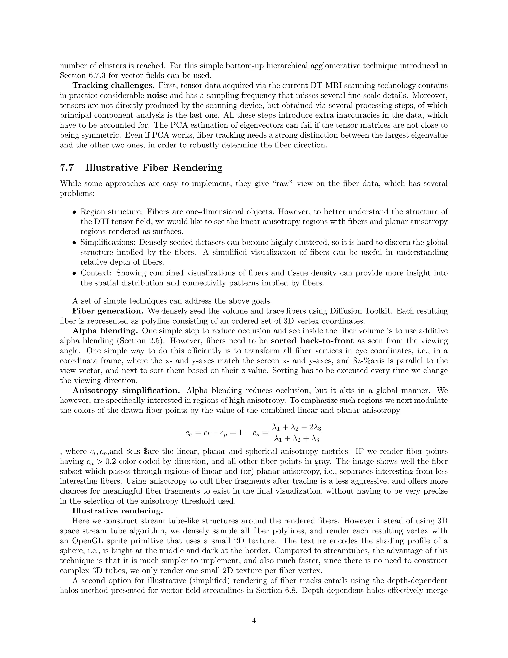
12. extension of IBFV that would be used to visualize 2D tensor fields. The idea is to use the major eigenvector
field to construct the IBFV animation, and, additionally, encode the minor eigenvector an (or) eigenvalue in
other attributes of the resulting visualization, such as color, luminance, or shading. How would you modify
IBFV to encode such additional attributes?
Hints: Take care that modifying luminance may adversely affect the result of IBFV, e.g., destroy the
apparent flow patterns that convey the direction of the major eigenvector field.
We can use same Noise texture advected in the direction of main eigenvector field. After obtaining
resulting texture N , we can color it based on orientation of the minor eigenvector.
13. EXERCISE 13
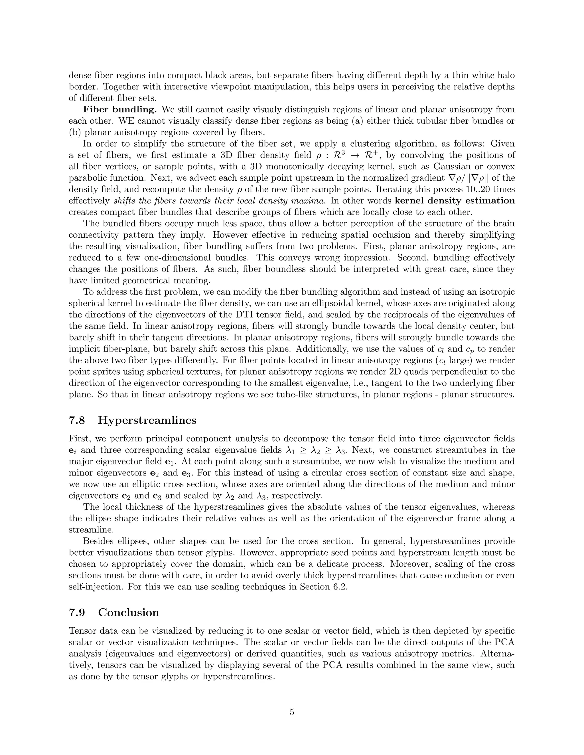
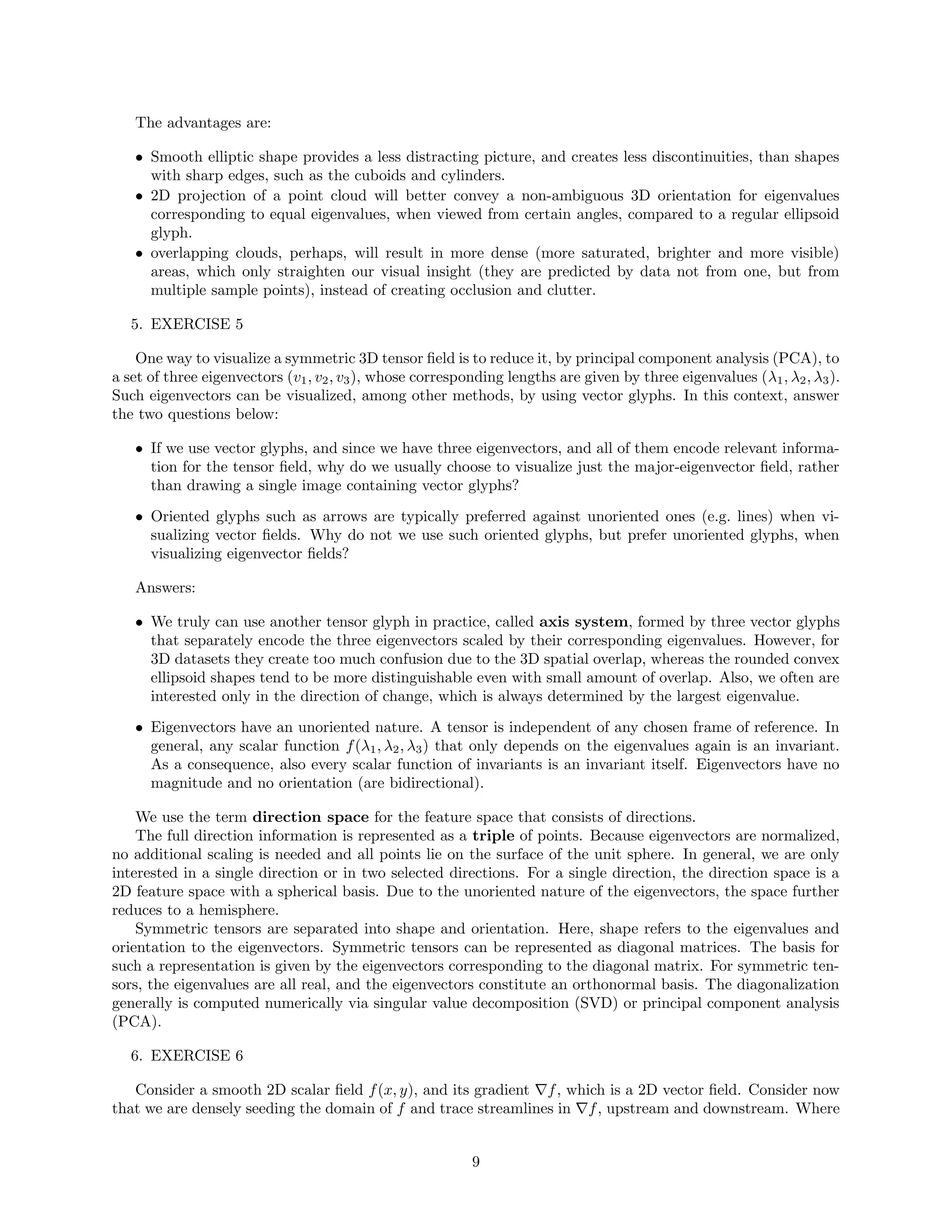
Consider a point cloud that densely samples a part of the surface of a sphere of radius R, defined in
polar coordinates θ, φ by the ranges [θmin, θmax] and [φmin, φmax]. The ‘patch’ created by this sampling is
shown in the figure below. Given the three points a, b, c indicated in the same figure, describe what are the
three eigenvectors of the principal component analysis (PCA) applied to the points’ covariance matrix for
small neighborhoods of each of these three points. The neighborhood sizes are indicated by the circles in the
figure. For this, indicate which are the directions of these eigenvectors, and (if possible from the provided
information), which are their relative magnitudes.
Figure 3: Point cloud sampling a sphere patch with three points of interest.
For the sphere λ1 = λ2 > 0. In this case we can only determine the minor eigenvector s3, and vectors s1
and s2 can be any two orthogonal vectors in the tangent plane, which are also orthogonal to s3.
Principal vector s3 is perpendicular to the tangent plane, and its magnitude equals λ3,and it coinsides
with the normal to abc plane at location C, when scaled by it’s corresponding eigenvalue: n = 1
λ3
s3.
Let’s define a centroid as follows:
C =
1
3
3
i=1
(pi − p) · (pi − p)T
, C · sj = λj · sj, j ∈ {1, 2, 3},
where k = 3 is the number of point-neighbors considered in the neighborhood of pi, so that p represents
the 3D centroid of the nearest neighbors, λj is the j-th eigenvalue of the covariance matrix, and sj the j-th
eigenvector.
12

13. PCA can yild following magnitudes for first two principal directions: λ1 = λ2 = r, so that r = |C − a| =
|C − b| = |C − c| is a radius of circumscribed circle of the triangle abc., and we can choose s1 = vecC − a,
(b,or c accordingly). Vector s2 = s⊥
1 belongs to plane abc and is orthogonal to s1 having same magnitude
|s2| = |s1| = r.
R = (sinθ cosϕ, sinθ sinϕ, cosθ)
Figure 4: Polar to Cartesian coordinate transformation in 3D.
13