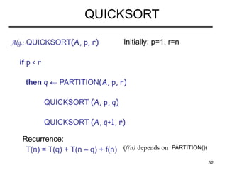
Quicksort is a divide-and-conquer sorting algorithm that works as follows:
1) Partition the array around a pivot element into two subarrays such that all elements in one subarray are less than or equal to the pivot and all elements in the other subarray are greater than the pivot.
2) Recursively sort the two subarrays.
3) The entire array is now sorted.
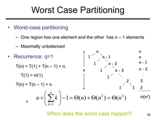
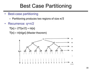
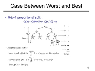
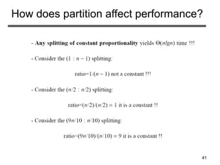
The performance of quicksort depends on how balanced the partition is - in the best case of a perfectly balanced partition, it runs in O(n log n) time, but in the worst case of a maximally unbalanced partition, it runs in O(n^2) time. The choice of

![5
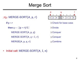
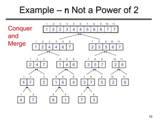
Merge Sort Approach
• To sort an array A[p . . r]:
• Divide
– Divide the n-element sequence to be sorted into two
subsequences of n/2 elements each
• Conquer
– Sort the subsequences recursively using merge sort
– When the size of the sequences is 1 there is nothing
more to do
• Combine
– Merge the two sorted subsequences](https://image.slidesharecdn.com/mergesortquicksort-230818014851-35b5cfb2/85/MergesortQuickSort-ppt-5-320.jpg)
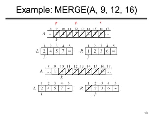
![11
Merging
• Input: Array A and indices p, q, r such that
p ≤ q < r
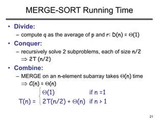
– Subarrays A[p . . q] and A[q + 1 . . r] are sorted
• Output: One single sorted subarray A[p . . r]
1 2 3 4 5 6 7 8
6
3
2
1
7
5
4
2
p r
q](https://image.slidesharecdn.com/mergesortquicksort-230818014851-35b5cfb2/85/MergesortQuickSort-ppt-11-320.jpg)
![12
Merging
• Idea for merging:
– Two piles of sorted cards
• Choose the smaller of the two top cards
• Remove it and place it in the output pile
– Repeat the process until one pile is empty
– Take the remaining input pile and place it face-down
onto the output pile
1 2 3 4 5 6 7 8
6
3
2
1
7
5
4
2
p r
q
A1 A[p, q]
A2 A[q+1, r]
A[p, r]](https://image.slidesharecdn.com/mergesortquicksort-230818014851-35b5cfb2/85/MergesortQuickSort-ppt-12-320.jpg)
![18
Merge - Pseudocode
Alg.: MERGE(A, p, q, r)
1. Compute n1 and n2
2. Copy the first n1 elements into
L[1 . . n1 + 1] and the next n2 elements into R[1 . . n2 + 1]
3. L[n1 + 1] ← ; R[n2 + 1] ←
4. i ← 1; j ← 1
5. for k ← p to r
6. do if L[ i ] ≤ R[ j ]
7. then A[k] ← L[ i ]
8. i ←i + 1
9. else A[k] ← R[ j ]
10. j ← j + 1
p q
7
5
4
2
6
3
2
1
r
q + 1
L
R
1 2 3 4 5 6 7 8
6
3
2
1
7
5
4
2
p r
q
n1 n2](https://image.slidesharecdn.com/mergesortquicksort-230818014851-35b5cfb2/85/MergesortQuickSort-ppt-18-320.jpg)
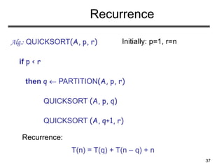
![30
Quicksort
• Sort an array A[p…r]
• Divide
– Partition the array A into 2 subarrays A[p..q] and A[q+1..r], such
that each element of A[p..q] is smaller than or equal to each
element in A[q+1..r]
– Need to find index q to partition the array
≤
A[p…q] A[q+1…r]](https://image.slidesharecdn.com/mergesortquicksort-230818014851-35b5cfb2/85/MergesortQuickSort-ppt-30-320.jpg)
![31
Quicksort
• Conquer
– Recursively sort A[p..q] and A[q+1..r] using Quicksort
• Combine
– Trivial: the arrays are sorted in place
– No additional work is required to combine them
– The entire array is now sorted
A[p…q] A[q+1…r]
≤](https://image.slidesharecdn.com/mergesortquicksort-230818014851-35b5cfb2/85/MergesortQuickSort-ppt-31-320.jpg)
![33
Partitioning the Array
• Choosing PARTITION()
– There are different ways to do this
– Each has its own advantages/disadvantages
• Hoare partition (see prob. 7-1, page 159)
– Select a pivot element x around which to partition
– Grows two regions
A[p…i] x
x A[j…r]
A[p…i] x x A[j…r]
i j](https://image.slidesharecdn.com/mergesortquicksort-230818014851-35b5cfb2/85/MergesortQuickSort-ppt-33-320.jpg)
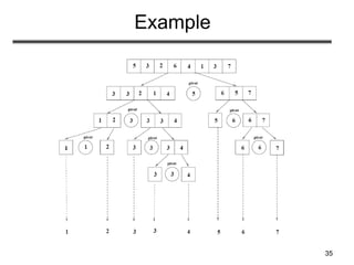
![34
Example
7
3
1
4
6
2
3
5
i j
7
5
1
4
6
2
3
3
i j
7
5
1
4
6
2
3
3
i j
7
5
6
4
1
2
3
3
i j
7
3
1
4
6
2
3
5
i j
A[p…r]
7
5
6
4
1
2
3
3
i
j
A[p…q] A[q+1…r]
pivot x=5](https://image.slidesharecdn.com/mergesortquicksort-230818014851-35b5cfb2/85/MergesortQuickSort-ppt-34-320.jpg)
![36
Partitioning the Array
Alg. PARTITION (A, p, r)
1. x A[p]
2. i p – 1
3. j r + 1
4. while TRUE
5. do repeat j j – 1
6. until A[j] ≤ x
7. do repeat i i + 1
8. until A[i] ≥ x
9. if i < j
10. then exchange A[i] A[j]
11. else return j
Running time: (n)
n = r – p + 1
7
3
1
4
6
2
3
5
i j
A:
ar
ap
i
j=q
A:
A[p…q] A[q+1…r]
≤
p r
Each element is
visited once!](https://image.slidesharecdn.com/mergesortquicksort-230818014851-35b5cfb2/85/MergesortQuickSort-ppt-36-320.jpg)


![UNIT V Searching Sorting Hashing Techniques [Autosaved].pptx](https://cdn.slidesharecdn.com/ss_thumbnails/unitvsearchingsortinghashingtechniquesautosaved-241126054304-95a69c51-thumbnail.jpg?width=640&height=640&fit=bounds)
![UNIT V Searching Sorting Hashing Techniques [Autosaved].pptx](https://cdn.slidesharecdn.com/ss_thumbnails/unitvsearchingsortinghashingtechniquesautosaved-241014040608-74caa0f6-thumbnail.jpg?width=640&height=640&fit=bounds)