DS2

1. Problem Solving Techniques and Data Structures

2. Course Objectives
2
• Problem Solving
Techniques
• Array, List, Stack, Queue
• Sorting Technique
• Searching Techniques
• Tree Data structure

3. www.hexaware.com | © Hexaware Technologies. All rights reserved. 52
Algorithm Design

4. Searching and Sorting
4
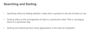
• Searching refers to finding whether a data item is present in the set of items or not
• Sorting refers to the arrangement of data in a particular order. That is, arranging
items in a particular way
• Sorting and searching have many applications in the area of computers

5. Searching Algorithms
5
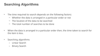
• The time required to search depends on the following factors:
– Whether the data is arranged in a particular order or not
– The location of the data to be searched
– The total number of searches to be done
• When the data is arranged in a particular order then, the time taken to search for
the item is less.
• Searching algorithms
– Linear Search
– Binary Search

6. www.hexaware.com | © Hexaware Technologies. All rights reserved. 55
Sorting Techniques

7. Sorting
7
• Arranging the data elements in a particular sequence – in the ascending
order (increasing order) or in the descending order (decreasing order)
• Sorting Algorithms:
– Selection Sort
– Insertion Sort
– Bubble Sort

8. Sorting
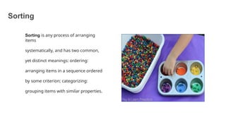
Sorting is any process of arranging
items
systematically, and has two common,
yet distinct meanings: ordering:
arranging items in a sequence ordered
by some criterion; categorizing:
grouping items with similar properties.
8

9. Sorting
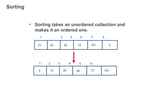
77 42 35 12 101 5
1 2 3 4 5 6
5 12 35 42 77 101
• Sorting takes an unordered collection and
makes it an ordered one.
1 2 3 4 5 6
9

10. Complexity of sorting Algorithm
10
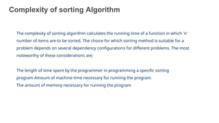
The complexity of sorting algorithm calculates the running time of a function in which 'n'
number of items are to be sorted. The choice for which sorting method is suitable for a
problem depends on several dependency configurations for different problems. The most
noteworthy of these considerations are:
The length of time spent by the programmer in programming a specific sorting
program Amount of machine time necessary for running the program
The amount of memory necessary for running the program

11. Types of Sorting Techniques
11
•Bubble Sort
•Selection
Sort
•Merge Sort
•Insertion
Sort
•Quick Sort

12. www.hexaware.com | © Hexaware Technologies. All rights reserved. 61
Bubble Sort

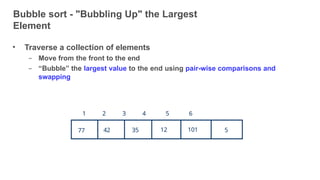
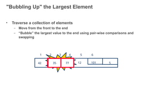
13. Bubble sort - "Bubbling Up" the Largest
Element
13
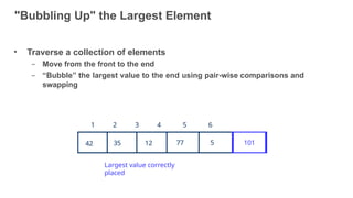
• Traverse a collection of elements
– Move from the front to the end
– “Bubble” the largest value to the end using pair-wise comparisons and
swapping
77 42 35 12 101 5
1 2 3 4 5 6

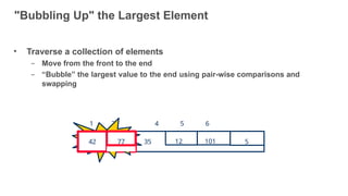
14. "Bubbling Up" the Largest Element
• Traverse a collection of elements
– Move from the front to the end
– “Bubble” the largest value to the end using pair-wise comparisons and
swapping
5
12
35 101
1 2
3
4 5 6
77 Swap42
42 77
14

15. "Bubbling Up" the Largest Element
• Traverse a collection of elements
– Move from the front to the end
– “Bubble” the largest value to the end using pair-wise comparisons and
swapping
5
12
42 101
1 2 3 4 5 6
77 Swap35
35 77
15

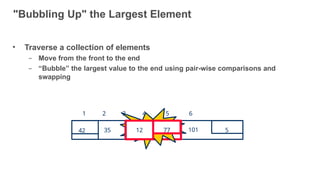
16. "Bubbling Up" the Largest Element
• Traverse a collection of elements
– Move from the front to the end
– “Bubble” the largest value to the end using pair-wise comparisons and
swapping
5
35
42 101
1 2 3 4 5 6
77 Swap
12
12
16
77

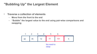
17. "Bubbling Up" the Largest Element
17
• Traverse a collection of elements
– Move from the front to the end
– “Bubble” the largest value to the end using pair-wise comparisons and
swapping
42 35 12 77 101 5
1 2 3 4 5 6
No need to
swap

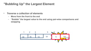
18. "Bubbling Up" the Largest Element
• Traverse a collection of elements
– Move from the front to the end
– “Bubble” the largest value to the end using pair-wise comparisons and
swapping
77
12
35
42
1 2 3
4
5 6
101 Sw
ap 5
5 101
18

19. "Bubbling Up" the Largest Element
Largest value correctly
placed
19
• Traverse a collection of elements
– Move from the front to the end
– “Bubble” the largest value to the end using pair-wise comparisons and
swapping
1 2 3 4 5 6
42 35 12 77 5 101

20. Items of Interest
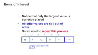
Largest value correctly
placed
20
• Notice that only the largest value is
correctly placed
• All other values are still out of
order
• So we need to repeat this process
1 2 3 4 5 6
42 35 12 77 5 101

21. Insertion sort
21

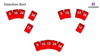
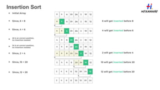
22. Insertion Sort
22
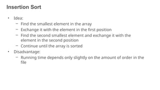
• Idea:
– Find the smallest element in the array
– Exchange it with the element in the first position
– Find the second smallest element and exchange it with the
element in the second position
– Continue until the array is sorted
• Disadvantage:
– Running time depends only slightly on the amount of order in the
file

23. Insertion Sort
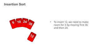
• To insert 12, we need to make
room for it by moving first 36
and then 24.
23

24. Insertion Sort
24

25. Insertion Sort
25

26. Selection sort
26

27. 76
27
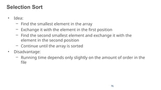
Selection Sort
• Idea:
– Find the smallest element in the array
– Exchange it with the element in the first position
– Find the second smallest element and exchange it with the
element in the second position
– Continue until the array is sorted
• Disadvantage:
– Running time depends only slightly on the amount of order in the
file

28. • Example: we are
given an array of six
integers that we want
to sort from smallest
to largest
70
60
50
40
30
20
10
0
[1] [2] [3] [4] [5] [6]
28
[0] [1] [2] [3] [4] [5]
Selection Sort

29. 70
60
50
40
30
20
10
0
• Start by finding
the
smallest entry.
29
[1] [2] [3] [4] [5] [6]
[0] [1] [2] [3] [4] [5]
Selection Sort

30. 79
70
60
50
40
30
20
10
0
• Swap the smallest
entry
with the first entry.
[1] [2] [3] [4] [5] [6]
[0] [1] [2] [3] [4] [5]
Selection Sort

31. 80
• Swap the smallest
entry with the first
entry.
70
60
50
40
30
20
10
0
[1] [2] [3] [4] [5] [6]
[0] [1] [2] [3] [4] [5]
Selection Sort

32. • Part of the array is
now
sorted.
70
60
50
40
30
20
10
0
[1] [2] [3] [4] [5] [6]
Sorted side Unsorted side
[0] [1]
32
[2] [3] [4] [5]
Selection Sort

33. 70
60
50
40
30
20
10
0
[1] [[22]] [[33]] [[44]] [[55]] [6]
• Find the smallest
element in the
unsorted side.
Sorted side Unsorted side
[0] [1]
33
[2] [3] [4] [5]
Selection Sort

34. 83
70
60
50
40
30
20
10
0
[1] [2] [3] [4] [5] [6]
• Swap with the front
of the unsorted
side.
Sorted side Unsorted side
[0] [1] [2] [3] [4] [5]
Selection Sort

35. 84
70
60
50
40
30
20
10
0
[1] [2] [3] [4] [5] [6]
• We have increased the
size of the sorted side
by one element.
Sorted side Unsorted side
[0] [1] [2] [3] [4] [5]
Selection Sort

36. 85
70
60
50
40
30
20
10
0
[1] [2] [3] [4] [5] [6]
• The
process
continues...
Sorted side Unsorted side
Smallest
from
unsorted
[0] [1] [2] [3] [4] [5]
Selection Sort

37. 70
60
50
40
30
20
10
0
[1] [2] [3] [4] [5] [6]
• The process
continues...
Sorted side Unsorted side
[0] [1] [2] [3] [4] [5]
Selection Sort
37

38. 70
60
50
40
30
20
10
0
[1] [2] [3] [4] [5] [6]
• The process
continues...
Sorted side Unsorted side
Sorted side
is bigger
[0] [1] [2] [3] [4] [5]
Selection Sort
38

39. 70
60
50
40
30
20
10
0
• The process keeps
adding one more
number to the
sorted side.
• The sorted side has
the smallest numbers,
arranged from small
to large.
Sorted side Unsorted side
[0] [1] [2] [3] [4] [5]
Selection Sort
[1] [2] [3] [4] [5]
[6][5] [6]
88

40. 70
60
50
40
30
20
10
0
[1] [2] [3] [4] [5] [6]
• We can stop when
the unsorted side has
just one number,
since that number
must be the largest
number.
[0] [1] [2] [3] [4] [5]
Sorted side Unsorted side
Selection Sort
40

41. Merge sort
41

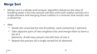
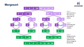
42. Merge Sort
2/19/0
3
42
42
• Merge sort is a divide-and-conquer algorithm based on the idea of
breaking down a list into several sub-lists until each sublist consists of a
single element and merging those sublists in a manner that results into
a sorted list.
• Idea:
• Divide the unsorted list into N sublists, each containing 1 element.
• Take adjacent pairs of two singleton lists and merge them to form a
list of 2
elements. N will now convert into N/2 lists of size 2.
• Repeat the process till a single sorted list of obtained.

43. “Divide and Conquer”
2/19/0
3
43
43
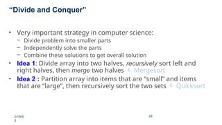
• Very important strategy in computer science:
– Divide problem into smaller parts
– Independently solve the parts
– Combine these solutions to get overall solution
• Idea 1: Divide array into two halves, recursively sort left and
right halves, then merge two halves  Mergesort
• Idea 2 : Partition array into items that are “small” and items
that are “large”, then recursively sort the two sets  Quicksort

44. 93
Mergesort
44

45. Quick sort
45

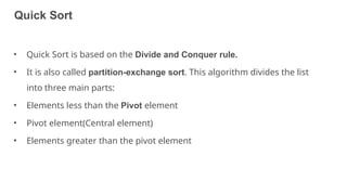
46. Quick Sort
46
• Quick Sort is based on the Divide and Conquer rule.
• It is also called partition-exchange sort. This algorithm divides the list
into three main parts:
• Elements less than the Pivot element
• Pivot element(Central element)
• Elements greater than the pivot element

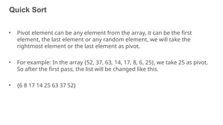
47. Quick Sort
47
• Pivot element can be any element from the array, it can be the first
element, the last element or any random element, we will take the
rightmost element or the last element as pivot.
• For example: In the array {52, 37, 63, 14, 17, 8, 6, 25}, we take 25 as pivot.
So after the first pass, the list will be changed like this.
• {6 8 17 14 25 63 37 52}

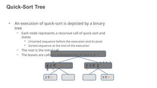
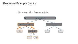
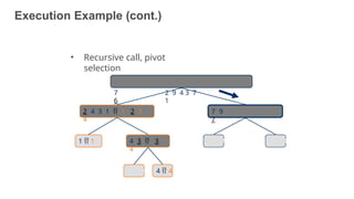
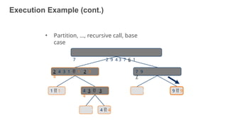
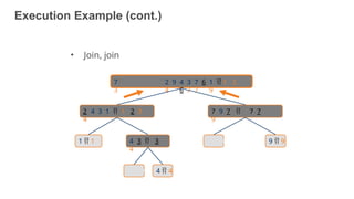
48. Quick-Sort Tree
• An execution of quick-sort is depicted by a binary
tree
– Each node represents a recursive call of quick-sort and
stores
• Unsorted sequence before the execution and its pivot
• Sorted sequence at the end of the execution
– The root is the initial call
– The leaves are calls on subsequences of size 0 or 1
7 4 9 6 2
 2 4 6 7
9
4 2  2
4
7 9  7
9
2  2 9  9
48

49. Execution Example
2
• Pivot selection
7
2 9
4 3
7 6
1
8
9 4
49

50. Execution Example (cont.)
2 4 3
1
9 4
• Partition, recursive call, pivot
selection
7 2 9 4 3 7 6 1
8
2
50

51. Execution Example (cont.)
2 4 3
1
1  1
9 4
• Partition, recursive call, base
case
7 2 9 4 3 7 6 1
8
51

52. Execution Example (cont.)
8
• Recursive call, …, base case, join
7 2 9 4 3 7 6 1
2 4 3 1  1 2 3
4
1  1 4 3  3
4
9 4  4
52

53. Execution Example (cont.)
7 9
7
8
• Recursive call, pivot
selection
7 2 9 4 3 7
6 1
2 4 3 1  1 2 3
4
1  1 4 3  3
4
9 4  4
9
53

54. Execution Example (cont.)
7 9
7
8
• Partition, …, recursive call, base
case
7 2 9 4 3 7 6 1
2 4 3 1  1 2 3
4
1  1 4 3  3
4
9 4  4
9  9
54

55. Execution Example (cont.)
7 9 7  7 7
9
8
• Join, join
7 2 9 4 3 7 6 1  1 2
3 4 6 7 7 9
2 4 3 1  1 2 3
4
1  1 4 3  3
4
9 4  4
9  9
55