Download to read offline
![28
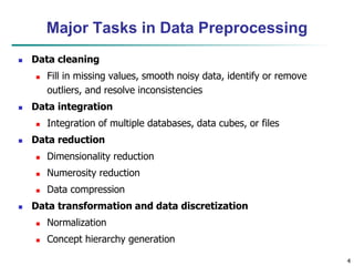
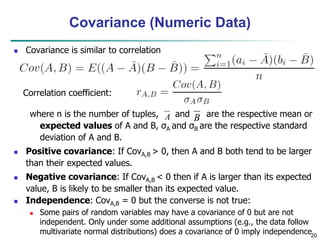
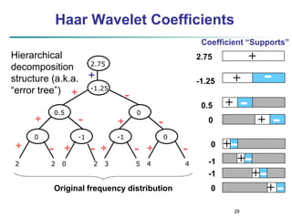
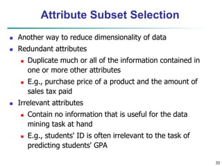
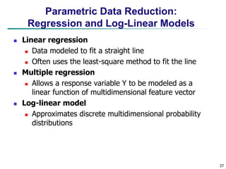
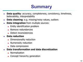
Wavelet Decomposition
Wavelets: A math tool for space-efficient hierarchical
decomposition of functions
S = [2, 2, 0, 2, 3, 5, 4, 4] can be transformed to S^ =
[23/4, -11/4, 1/2, 0, 0, -1, -1, 0]
Compression: many small detail coefficients can be
replaced by 0’s, and only the significant coefficients are
retained](https://image.slidesharecdn.com/chapter3-230924172505-6d42a8a0/85/Chapter-3-Data-Preprocessing-ppt-28-320.jpg)
![51
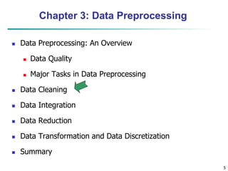
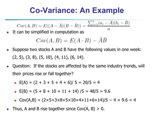
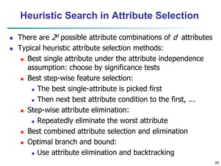
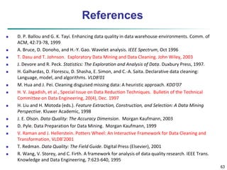
Normalization
Min-max normalization: to [new_minA, new_maxA]
Ex. Let income range $12,000 to $98,000 normalized to [0.0,
1.0]. Then $73,000 is mapped to
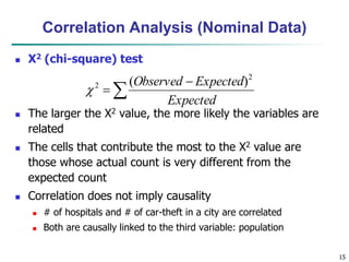
Z-score normalization (μ: mean, σ: standard deviation):
Ex. Let μ = 54,000, σ = 16,000. Then
Normalization by decimal scaling
716
.
0
0
)
0
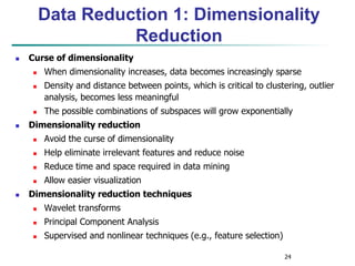
0
.
1
(
000
,
12
000
,
98
000
,
12
600
,
73
A
A
A
A
A
A
min
new
min
new
max
new
min
max
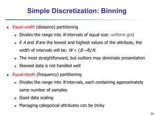
min
v
v _
)
_
_
(
'
A
A
v
v
'
j
v
v
10
' Where j is the smallest integer such that Max(|ν’|) < 1
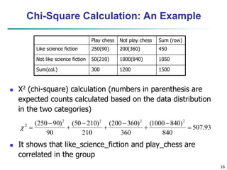
225
.
1
000
,
16
000
,
54
600
,
73
](https://image.slidesharecdn.com/chapter3-230924172505-6d42a8a0/85/Chapter-3-Data-Preprocessing-ppt-51-320.jpg)
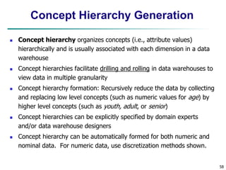

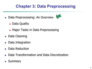
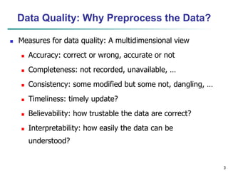
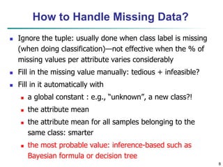
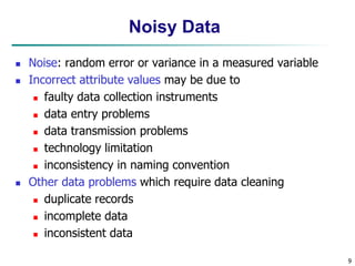
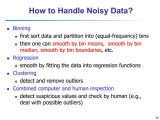
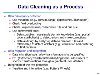
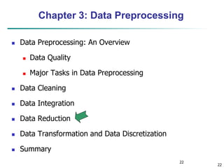
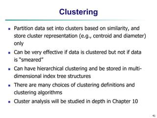
Chapter 3 focuses on data preprocessing, outlining its importance in ensuring data quality through major tasks such as data cleaning, integration, reduction, and transformation. It discusses strategies for managing missing and noisy data and methods for dimensionality reduction, including techniques like principal component analysis and wavelet transforms. The chapter emphasizes the necessity of data preprocessing for enhancing the efficiency and effectiveness of data mining operations.