DATA MINING
LECTURE 13
Absorbing Random walks
Coverage
Subrata Kumer Paul
Assistant Professor, Dept. of CSE, BAUET
sksubrata96@gmail.com
ABSORBING RANDOM
WALKS
Random walk with absorbing nodes
• What happens if we do a random walk on this
graph? What is the stationary distribution?
• All the probability mass on the red sink node:
• The red node is an absorbing node
Random walk with absorbing nodes
• What happens if we do a random walk on this graph?
What is the stationary distribution?
• There are two absorbing nodes: the red and the blue.
• The probability mass will be divided between the two
Absorption probability
• If there are more than one absorbing nodes in the
graph a random walk that starts from a non-
absorbing node will be absorbed in one of them
with some probability
• The probability of absorption gives an estimate of how
close the node is to red or blue
Absorption probability
• Computing the probability of being absorbed:
• The absorbing nodes have probability 1 of being absorbed in
themselves and zero of being absorbed in another node.
• For the non-absorbing nodes, take the (weighted) average of
the absorption probabilities of your neighbors
• if one of the neighbors is the absorbing node, it has probability 1
• Repeat until convergence (= very small change in probs)
𝑃 𝑅𝑒𝑑 𝑃𝑖𝑛𝑘 =
2
3
𝑃 𝑅𝑒𝑑 𝑌𝑒𝑙𝑙𝑜𝑤 +
1
3
𝑃(𝑅𝑒𝑑|𝐺𝑟𝑒𝑒𝑛)
𝑃 𝑅𝑒𝑑 𝐺𝑟𝑒𝑒𝑛 =
1
4
𝑃 𝑅𝑒𝑑 𝑌𝑒𝑙𝑙𝑜𝑤 +
1
4
𝑃 𝑅𝑒𝑑 𝑌𝑒𝑙𝑙𝑜𝑤 =
2
3
2
2
1
1
1
2
1
Absorption probability
• Computing the probability of being absorbed:
• The absorbing nodes have probability 1 of being absorbed in
themselves and zero of being absorbed in another node.
• For the non-absorbing nodes, take the (weighted) average of
the absorption probabilities of your neighbors
• if one of the neighbors is the absorbing node, it has probability 1
• Repeat until convergence (= very small change in probs)
𝑃 𝐵𝑙𝑢𝑒 𝑃𝑖𝑛𝑘 =
2
3
𝑃 𝐵𝑙𝑢𝑒 𝑌𝑒𝑙𝑙𝑜𝑤 +
1
3
𝑃(𝐵𝑙𝑢𝑒|𝐺𝑟𝑒𝑒𝑛)
𝑃 𝐵𝑙𝑢𝑒 𝐺𝑟𝑒𝑒𝑛 =
1
4
𝑃 𝐵𝑙𝑢𝑒 𝑌𝑒𝑙𝑙𝑜𝑤 +
1
2
𝑃 𝐵𝑙𝑢𝑒 𝑌𝑒𝑙𝑙𝑜𝑤 =
1
3
2
2
1
1
1
2
1
Why do we care?
• Why do we care to compute the absorption
probability to sink nodes?
• Given a graph (directed or undirected) we can
choose to make some nodes absorbing.
• Simply direct all edges incident on the chosen nodes towards
them and remove outgoing edges.
• The absorbing random walk provides a measure of
proximity of non-absorbing nodes to the chosen
nodes.
• Useful for understanding proximity in graphs
• Useful for propagation in the graph
• E.g, some nodes have positive opinions for an issue, some have
negative, to which opinion is a non-absorbing node closer?
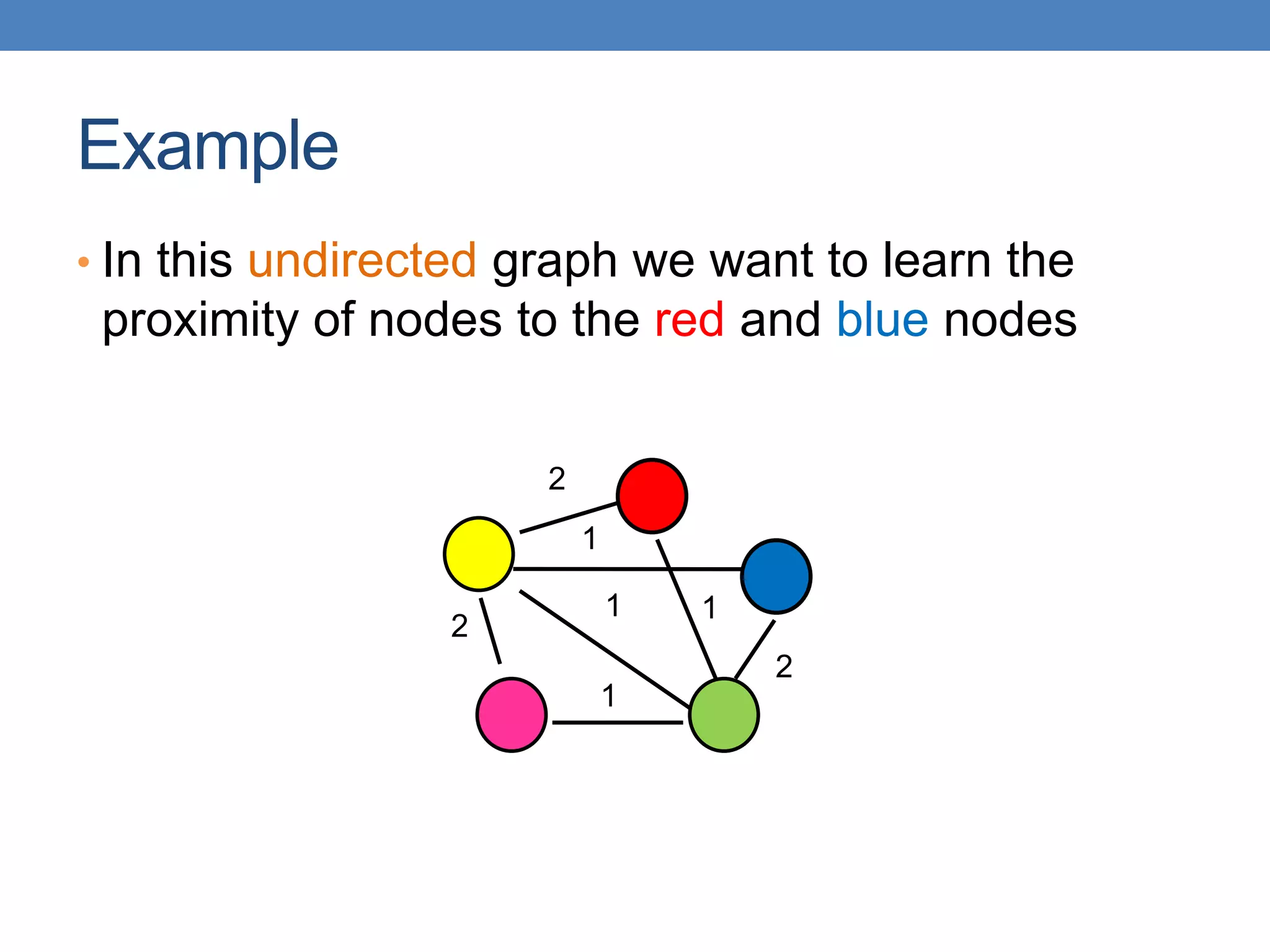
Example
• In this undirected graph we want to learn the
proximity of nodes to the red and blue nodes
2
2
1
1
1
2
1
Example
• Make the nodes absorbing
2
2
1
1
1
2
1
Absorption probability
• Compute the absorbtion probabilities for red and
blue
𝑃 𝑅𝑒𝑑 𝑃𝑖𝑛𝑘 =
2
3
𝑃 𝑅𝑒𝑑 𝑌𝑒𝑙𝑙𝑜𝑤 +
1
3
𝑃(𝑅𝑒𝑑|𝐺𝑟𝑒𝑒𝑛)
𝑃 𝑅𝑒𝑑 𝐺𝑟𝑒𝑒𝑛 =
1
5
𝑃 𝑅𝑒𝑑 𝑌𝑒𝑙𝑙𝑜𝑤 +
1
5
𝑃 𝑅𝑒𝑑 𝑃𝑖𝑛𝑘 +
1
5
𝑃 𝑅𝑒𝑑 𝑌𝑒𝑙𝑙𝑜𝑤 =
1
6
𝑃 𝑅𝑒𝑑 𝐺𝑟𝑒𝑒𝑛 +
1
3
𝑃 𝑅𝑒𝑑 𝑃𝑖𝑛𝑘 +
1
3
0.52
0.48
0.42
0.58
0.57
0.43 2
2
1
1
1
2
1
𝑃 𝐵𝑙𝑢𝑒 𝑃𝑖𝑛𝑘 = 1 − 𝑃 𝑅𝑒𝑑 𝑃𝑖𝑛𝑘
𝑃 𝐵𝑙𝑢𝑒 𝐺𝑟𝑒𝑒𝑛 = 1 − 𝑃 𝑅𝑒𝑑 𝐺𝑟𝑒𝑒𝑛
𝑃 𝐵𝑙𝑢𝑒 𝑌𝑒𝑙𝑙𝑜𝑤 = 1 − 𝑃 𝑅𝑒𝑑 𝑌𝑒𝑙𝑙𝑜𝑤
Penalizing long paths
• The orange node has the same probability of
reaching red and blue as the yellow one
• Intuitively though it is further away
0.52
0.48
0.42
0.58
0.57
0.43 2
2
1
1
1
2
1
𝑃 𝐵𝑙𝑢𝑒 𝑂𝑟𝑎𝑛𝑔𝑒 = 𝑃 𝐵𝑙𝑢𝑒 𝑌𝑒𝑙𝑙𝑜𝑤 1
𝑃 𝑅𝑒𝑑 𝑂𝑟𝑎𝑛𝑔𝑒 = 𝑃 𝑅𝑒𝑑 𝑌𝑒𝑙𝑙𝑜𝑤
0.57
0.43
Penalizing long paths
• Add an universal absorbing node to which each
node gets absorbed with probability α.
1-α
α
α
α α
1-α
1-α
1-α
𝑃 𝑅𝑒𝑑 𝐺𝑟𝑒𝑒𝑛 = (1 − 𝛼)
1
5
𝑃 𝑅𝑒𝑑 𝑌𝑒𝑙𝑙𝑜𝑤 +
1
5
𝑃 𝑅𝑒𝑑 𝑃𝑖𝑛𝑘 +
1
5
With probability α the random walk dies
With probability (1-α) the random walk
continues as before
The longer the path from a node to an
absorbing node the more likely the random
walk dies along the way, the lower the
absorbtion probability
e.g.
Random walk with restarts
• Adding a jump with probability α to a universal absorbing node
seems similar to Pagerank
• Random walk with restart:
• Start a random walk from node u
• At every step with probability α, jump back to u
• The probability of being at node v after large number of steps defines again a
similarity between u,v
• The Random Walk With Restarts (RWS) and Absorbing Random
Walk (ARW) are similar but not the same
• RWS computes the probability of paths from the starting node u to a node v,
while AWR the probability of paths from a node v, to the absorbing node u.
• RWS defines a distribution over all nodes, while AWR defines a probability for
each node
• An absorbing node blocks the random walk, while restarts simply bias towards
starting nodes
• Makes a difference when having multiple (and possibly competing) absorbing nodes
Propagating values
• Assume that Red has a positive value and Blue a
negative value
• Positive/Negative class, Positive/Negative opinion
• We can compute a value for all the other nodes by
repeatedly averaging the values of the neighbors
• The value of node u is the expected value at the point of absorption
for a random walk that starts from u
𝑉(𝑃𝑖𝑛𝑘) =
2
3
𝑉(𝑌𝑒𝑙𝑙𝑜𝑤) +
1
3
𝑉(𝐺𝑟𝑒𝑒𝑛)
𝑉 𝐺𝑟𝑒𝑒𝑛 =
1
5
𝑉(𝑌𝑒𝑙𝑙𝑜𝑤) +
1
5
𝑉(𝑃𝑖𝑛𝑘) +
1
5
−
2
5
𝑉 𝑌𝑒𝑙𝑙𝑜𝑤 =
1
6
𝑉 𝐺𝑟𝑒𝑒𝑛 +
1
3
𝑉(𝑃𝑖𝑛𝑘) +
1
3
−
1
6
+1
-1
0.05 -0.16
0.16 2
2
1
1
1
2
1
Electrical networks and random walks
• Our graph corresponds to an electrical network
• There is a positive voltage of +1 at the Red node, and a
negative voltage -1 at the Blue node
• There are resistances on the edges inversely proportional to
the weights (or conductance proportional to the weights)
• The computed values are the voltages at the nodes
+1
𝑉(𝑃𝑖𝑛𝑘) =
2
3
𝑉(𝑌𝑒𝑙𝑙𝑜𝑤) +
1
3
𝑉(𝐺𝑟𝑒𝑒𝑛)
𝑉 𝐺𝑟𝑒𝑒𝑛 =
1
5
𝑉(𝑌𝑒𝑙𝑙𝑜𝑤) +
1
5
𝑉(𝑃𝑖𝑛𝑘) +
1
5
−
2
5
𝑉 𝑌𝑒𝑙𝑙𝑜𝑤 =
1
6
𝑉 𝐺𝑟𝑒𝑒𝑛 +
1
3
𝑉(𝑃𝑖𝑛𝑘) +
1
3
−
1
6
+1
-1
2
2
1
1
1
2
1
0.05 -0.16
0.16
Opinion formation
• The value propagation can be used as a model of opinion formation.
• Model:
• Opinions are values in [-1,1]
• Every user 𝑢 has an internal opinion 𝑠𝑢, and expressed opinion 𝑧𝑢.
• The expressed opinion minimizes the personal cost of user 𝑢:
𝑐 𝑧𝑢 = 𝑠𝑢 − 𝑧𝑢
2
+
𝑣:𝑣 is a friend of 𝑢
𝑤𝑢 𝑧𝑢 − 𝑧𝑣
2
• Minimize deviation from your beliefs and conflicts with the society
• If every user tries independently (selfishly) to minimize their personal
cost then the best thing to do is to set 𝑧𝑢to the average of all opinions:
𝑧𝑢 =
𝑠𝑢 + 𝑣:𝑣 is a friend of 𝑢 𝑤𝑢𝑧𝑢
1 + 𝑣:𝑣 is a friend of 𝑢 𝑤𝑢
• This is the same as the value propagation we described before!
Example
• Social network with internal opinions
2
2
1
1
1
2
1
s = +0.5
s = -0.3
s = -0.1
s = +0.2
s = +0.8
Example
2
2
1
1
1
2
1
1
1
1 1
1
s = +0.5
s = -0.3
s = -0.1
s = -0.5
s = +0.8
The external opinion for each node is
computed using the value propagation
we described before
• Repeated averaging
Intuitive model: my opinion is a
combination of what I believe and
what my social network believes.
One absorbing node per user with
value the internal opinion of the user
One non-absorbing node per user
that links to the corresponding
absorbing node
z = +0.22
z = +0.17
z = -0.03
z = 0.04
z = -0.01
Hitting time
• A related quantity: Hitting time H(u,v)
• The expected number of steps for a random walk
starting from node u to end up in v for the first time
• Make node v absorbing and compute the expected number of
steps to reach v
• Assumes that the graph is strongly connected, and there are no
other absorbing nodes.
• Commute time H(u,v) + H(v,u): often used as a
distance metric
• Proportional to the total resistance between nodes u,
and v
Transductive learning
• If we have a graph of relationships and some labels on some
nodes we can propagate them to the remaining nodes
• Make the labeled nodes to be absorbing and compute the probability
for the rest of the graph
• E.g., a social network where some people are tagged as spammers
• E.g., the movie-actor graph where some movies are tagged as action
or comedy.
• This is a form of semi-supervised learning
• We make use of the unlabeled data, and the relationships
• It is also called transductive learning because it does not
produce a model, but just labels the unlabeled data that is at
hand.
• Contrast to inductive learning that learns a model and can label any
new example
Implementation details
• Implementation is in many ways similar to the
PageRank implementation
• For an edge (𝑢, 𝑣)instead of updating the value of v we
update the value of u.
• The value of a node is the average of its neighbors
• We need to check for the case that a node u is
absorbing, in which case the value of the node is not
updated.
• Repeat the updates until the change in values is very
small.
COVERAGE
Example
• Promotion campaign on a social network
• We have a social network as a graph.
• People are more likely to buy a product if they have a friend who
has the product.
• We want to offer the product for free to some people such that
every person in the graph is covered: they have a friend who has
the product.
• We want the number of free products to be as small as possible
Example
One possible selection
• Promotion campaign on a social network
• We have a social network as a graph.
• People are more likely to buy a product if they have a friend who
has the product.
• We want to offer the product for free to some people such that
every person in the graph is covered: they have a friend who has
the product.
• We want the number of free products to be as small as possible
Example
A better selection
• Promotion campaign on a social network
• We have a social network as a graph.
• People are more likely to buy a product if they have a friend who
has the product.
• We want to offer the product for free to some people such that
every person in the graph is covered: they have a friend who has
the product.
• We want the number of free products to be as small as possible
Dominating set
• Our problem is an instance of the dominating set
problem
• Dominating Set: Given a graph 𝐺 = (𝑉, 𝐸), a set
of vertices 𝐷 ⊆ 𝑉 is a dominating set if for each
node u in V, either u is in D, or u has a neighbor
in D.
• The Dominating Set Problem: Given a graph 𝐺 =
(𝑉, 𝐸) find a dominating set of minimum size.
Set Cover
• The dominating set problem is a special case of
the Set Cover problem
• The Set Cover problem:
• We have a universe of elements 𝑈 = 𝑥1, … , 𝑥𝑁
• We have a collection of subsets of U, 𝑺 = {𝑆1, … , 𝑆𝑛},
such that 𝑖 𝑆𝑖 = 𝑈
• We want to find the smallest sub-collection 𝑪 ⊆ 𝑺 of 𝑺,
such that 𝑆𝑖∈𝑪 𝑆𝑖 = 𝑈
• The sets in 𝑪 cover the elements of U
Applications
• Dominating Set (or Promotion Campaign) as Set
Cover:
• The universe U is the set of nodes V
• Each node 𝑢 defines a set 𝑆𝑢 consisting of the node 𝑢 and all
of its neighbors
• We want the minimum number of sets 𝑆𝑢 (nodes) that cover
all the nodes in the graph.
• Another example: Document summarization
• A document consists of a set of terms T (the universe U of
elements), and a set of sentences S, where each sentence is
a set of terms.
• Find the smallest set of sentences C, that cover all the terms
in the document.
• Many more…
Best selection variant
• Suppose that we have a budget K of how big our
set cover can be
• We only have K products to give out for free.
• We want to cover as many customers as possible.
• Maximum-Coverage Problem: Given a universe
of elements U, a collection of S of subsets of U,
and a budget K, find a sub-collection 𝑪 ⊆ 𝑺 of
size K, such that the number of covered elemets
𝑆𝑖∈𝑪 𝑆𝑖 is maximized.
Complexity
• Both the Set Cover and the Maximum Coverage
problems are NP-complete
• What does this mean?
• Why do we care?
• There is no algorithm that can guarantee to find
the best solution in polynomial time
• Can we find an algorithm that can guarantee to find a
solution that is close to the optimal?
• Approximation Algorithms.
Approximation Algorithms
• For an (combinatorial) optimization problem, where:
• X is an instance of the problem,
• OPT(X) is the value of the optimal solution for X,
• ALG(X) is the value of the solution of an algorithm ALG for X
ALG is a good approximation algorithm if the ratio of OPT(X) and
ALG(X) is bounded for all input instances X
• Minimum set cover: X = G is the input graph, OPT(G) is the
size of minimum set cover, ALG(G) is the size of the set cover
found by an algorithm ALG.
• Maximum coverage: X = (G,k) is the input instance, OPT(G,k)
is the coverage of the optimal algorithm, ALG(G,k) is the
coverage of the set found by an algorithm ALG.
Approximation Algorithms
• For a minimization problem, the algorithm ALG is
an 𝛼-approximation algorithm, for 𝛼 > 1, if for all
input instances X,
𝐴𝐿𝐺 𝑋 ≤ 𝛼𝑂𝑃𝑇 𝑋
• 𝛼 is the approximation ratio of the algorithm – we
want 𝛼 to be as close to 1 as possible
• Best case: 𝛼 = 1 + 𝜖 and 𝜖 → 0, as 𝑛 → ∞ (e.g., 𝜖 =
1
𝑛
)
• Good case: 𝛼 = 𝑂(1) is a constant
• OK case: 𝛼 = O(log 𝑛)
• Bad case 𝛼 = O( 𝑛𝜖
)
Approximation Algorithms
• For a maximization problem, the algorithm ALG is an
𝛼-approximation algorithm, for 𝛼 < 1, if for all input
instances X,
𝐴𝐿𝐺 𝑋 ≥ 𝛼𝑂𝑃𝑇 𝑋
• 𝛼 is the approximation ratio of the algorithm – we
want 𝛼 to be as close to 1 as possible
• Best case: 𝛼 = 1 − 𝜖 and 𝜖 → 0, as 𝑛 → ∞(e.g., 𝜖 =
1
𝑛
)
• Good case: 𝛼 = 𝑂(1) is a constant
• OK case: 𝛼 = 𝑂(
1
log 𝑛
)
• Bad case 𝛼 = O( 𝑛−𝜖)
A simple approximation ratio for set cover
• Any algorithm for set cover has approximation
ratio  = |Smax|, where Smax is the set in S with the
largest cardinality
• Proof:
• OPT(X)≥N/|Smax|  N ≤ |Smax|OPT(X)
• ALG(X) ≤ N ≤ |Smax|OPT(X)
• This is true for any algorithm.
• Not a good bound since it can be that |Smax|=O(N)
An algorithm for Set Cover
• What is the most natural algorithm for Set Cover?
• Greedy: each time add to the collection C the set
Si from S that covers the most of the remaining
elements.
The GREEDY algorithm
GREEDY(U,S)
X= U
C = {}
while X is not empty do
For all 𝑆𝑖 ∈ 𝑺 let gain(𝑆𝑖) = |𝑆𝑖 ∩ 𝑋|
Let 𝑆∗be such that 𝑔𝑎𝑖𝑛(𝑆∗) is maximum
C = C U {S*}
X = X S*
S = S S*
Approximation ratio of GREEDY
• Good news: GREEDY has approximation ratio:
𝛼 = 𝐻 𝑆max = 1 + ln 𝑆max , 𝐻 𝑛 =
𝑘=1
𝑛
1
𝑘
𝐺𝑅𝐸𝐸𝐷𝑌 𝑋 ≤ 1 + ln 𝑆max 𝑂𝑃𝑇 𝑋 , for all X
• The approximation ratio is tight up to a constant
• Tight means that we can find a counter example with this ratio
OPT(X) = 2
GREEDY(X) = logN
=½logN
Maximum Coverage
• What is a reasonable algorithm?
GREEDY(U,S,K)
X = U
C = {}
while |C| < K
For all 𝑆𝑖 ∈ 𝑺 let gain(𝑆𝑖) = |𝑆𝑖 ∩ 𝑋|
Let 𝑆∗ be such that 𝑔𝑎𝑖𝑛(𝑆∗) is maximum
C = C U {S*}
X = X S*
S= S S*
Approximation Ratio for Max-K Coverage
• Better news! The GREEDY algorithm has
approximation ratio 𝛼 = 1 −
1
𝑒
𝐺𝑅𝐸𝐸𝐷𝑌 𝑋 ≥ 1 −
1
𝑒
𝑂𝑃𝑇 𝑋 , for all X
• The coverage of the Greedy solution is at least
63% that of the optimal
Proof of approximation ratio
• For a collection C, let 𝐹 𝐶 = 𝑆𝑖∈𝑪 𝑆𝑖 be the number of
elements that are covered.
• The function F has two properties:
• F is monotone:
𝐹 𝐴 ≤ 𝐹 𝐵 𝑖𝑓 𝐴 ⊆ 𝐵
• F is submodular:
𝐹 𝐴 ∪ 𝑆 − 𝐹 𝐴 ≥ 𝐹 𝐵 ∪ 𝑆 − 𝐹 𝐵 𝑖𝑓 𝐴 ⊆ 𝐵
• The addition of set 𝑆 to a set of nodes has greater effect
(more new covered items) for a smaller set.
• The diminishing returns property
Optimizing submodular functions
• Theorem: A greedy algorithm that optimizes a
monotone and submodular function F, each time
adding to the solution C, the set S that maximizes
the gain 𝐹 𝐶 ∪ 𝑆 − 𝐹(𝐶) has approximation
ratio 𝛼 = 1 −
1
𝑒
Other variants of Set Cover
• Hitting Set: select a set of elements so that you
hit all the sets (the same as the set cover,
reversing the roles)
• Vertex Cover: Select a subset of vertices such
that you cover all edges (an endpoint of each
edge is in the set)
• There is a 2-approximation algorithm
• Edge Cover: Select a set of edges that cover all
vertices (there is one edge that has endpoint the
vertex)
• There is a polynomial algorithm
Parting thoughts
• In this class you saw a set of tools for analyzing data
• Association Rules
• Sketching
• Clustering
• Minimum Description Length
• Signular Value Decomposition
• Classification
• Random Walks
• Coverage
• All these are useful when trying to make sense of the
data. A lot more tools exist.
• I hope that you found this interesting, useful and fun.

Data Mining Lecture_13.pptx

  • 1.
    DATA MINING LECTURE 13 AbsorbingRandom walks Coverage Subrata Kumer Paul Assistant Professor, Dept. of CSE, BAUET sksubrata96@gmail.com
  • 2.
  • 3.
    Random walk withabsorbing nodes • What happens if we do a random walk on this graph? What is the stationary distribution? • All the probability mass on the red sink node: • The red node is an absorbing node
  • 4.
    Random walk withabsorbing nodes • What happens if we do a random walk on this graph? What is the stationary distribution? • There are two absorbing nodes: the red and the blue. • The probability mass will be divided between the two
  • 5.
    Absorption probability • Ifthere are more than one absorbing nodes in the graph a random walk that starts from a non- absorbing node will be absorbed in one of them with some probability • The probability of absorption gives an estimate of how close the node is to red or blue
  • 6.
    Absorption probability • Computingthe probability of being absorbed: • The absorbing nodes have probability 1 of being absorbed in themselves and zero of being absorbed in another node. • For the non-absorbing nodes, take the (weighted) average of the absorption probabilities of your neighbors • if one of the neighbors is the absorbing node, it has probability 1 • Repeat until convergence (= very small change in probs) 𝑃 𝑅𝑒𝑑 𝑃𝑖𝑛𝑘 = 2 3 𝑃 𝑅𝑒𝑑 𝑌𝑒𝑙𝑙𝑜𝑤 + 1 3 𝑃(𝑅𝑒𝑑|𝐺𝑟𝑒𝑒𝑛) 𝑃 𝑅𝑒𝑑 𝐺𝑟𝑒𝑒𝑛 = 1 4 𝑃 𝑅𝑒𝑑 𝑌𝑒𝑙𝑙𝑜𝑤 + 1 4 𝑃 𝑅𝑒𝑑 𝑌𝑒𝑙𝑙𝑜𝑤 = 2 3 2 2 1 1 1 2 1
  • 7.
    Absorption probability • Computingthe probability of being absorbed: • The absorbing nodes have probability 1 of being absorbed in themselves and zero of being absorbed in another node. • For the non-absorbing nodes, take the (weighted) average of the absorption probabilities of your neighbors • if one of the neighbors is the absorbing node, it has probability 1 • Repeat until convergence (= very small change in probs) 𝑃 𝐵𝑙𝑢𝑒 𝑃𝑖𝑛𝑘 = 2 3 𝑃 𝐵𝑙𝑢𝑒 𝑌𝑒𝑙𝑙𝑜𝑤 + 1 3 𝑃(𝐵𝑙𝑢𝑒|𝐺𝑟𝑒𝑒𝑛) 𝑃 𝐵𝑙𝑢𝑒 𝐺𝑟𝑒𝑒𝑛 = 1 4 𝑃 𝐵𝑙𝑢𝑒 𝑌𝑒𝑙𝑙𝑜𝑤 + 1 2 𝑃 𝐵𝑙𝑢𝑒 𝑌𝑒𝑙𝑙𝑜𝑤 = 1 3 2 2 1 1 1 2 1
  • 8.
    Why do wecare? • Why do we care to compute the absorption probability to sink nodes? • Given a graph (directed or undirected) we can choose to make some nodes absorbing. • Simply direct all edges incident on the chosen nodes towards them and remove outgoing edges. • The absorbing random walk provides a measure of proximity of non-absorbing nodes to the chosen nodes. • Useful for understanding proximity in graphs • Useful for propagation in the graph • E.g, some nodes have positive opinions for an issue, some have negative, to which opinion is a non-absorbing node closer?
  • 9.
    Example • In thisundirected graph we want to learn the proximity of nodes to the red and blue nodes 2 2 1 1 1 2 1
  • 10.
    Example • Make thenodes absorbing 2 2 1 1 1 2 1
  • 11.
    Absorption probability • Computethe absorbtion probabilities for red and blue 𝑃 𝑅𝑒𝑑 𝑃𝑖𝑛𝑘 = 2 3 𝑃 𝑅𝑒𝑑 𝑌𝑒𝑙𝑙𝑜𝑤 + 1 3 𝑃(𝑅𝑒𝑑|𝐺𝑟𝑒𝑒𝑛) 𝑃 𝑅𝑒𝑑 𝐺𝑟𝑒𝑒𝑛 = 1 5 𝑃 𝑅𝑒𝑑 𝑌𝑒𝑙𝑙𝑜𝑤 + 1 5 𝑃 𝑅𝑒𝑑 𝑃𝑖𝑛𝑘 + 1 5 𝑃 𝑅𝑒𝑑 𝑌𝑒𝑙𝑙𝑜𝑤 = 1 6 𝑃 𝑅𝑒𝑑 𝐺𝑟𝑒𝑒𝑛 + 1 3 𝑃 𝑅𝑒𝑑 𝑃𝑖𝑛𝑘 + 1 3 0.52 0.48 0.42 0.58 0.57 0.43 2 2 1 1 1 2 1 𝑃 𝐵𝑙𝑢𝑒 𝑃𝑖𝑛𝑘 = 1 − 𝑃 𝑅𝑒𝑑 𝑃𝑖𝑛𝑘 𝑃 𝐵𝑙𝑢𝑒 𝐺𝑟𝑒𝑒𝑛 = 1 − 𝑃 𝑅𝑒𝑑 𝐺𝑟𝑒𝑒𝑛 𝑃 𝐵𝑙𝑢𝑒 𝑌𝑒𝑙𝑙𝑜𝑤 = 1 − 𝑃 𝑅𝑒𝑑 𝑌𝑒𝑙𝑙𝑜𝑤
  • 12.
    Penalizing long paths •The orange node has the same probability of reaching red and blue as the yellow one • Intuitively though it is further away 0.52 0.48 0.42 0.58 0.57 0.43 2 2 1 1 1 2 1 𝑃 𝐵𝑙𝑢𝑒 𝑂𝑟𝑎𝑛𝑔𝑒 = 𝑃 𝐵𝑙𝑢𝑒 𝑌𝑒𝑙𝑙𝑜𝑤 1 𝑃 𝑅𝑒𝑑 𝑂𝑟𝑎𝑛𝑔𝑒 = 𝑃 𝑅𝑒𝑑 𝑌𝑒𝑙𝑙𝑜𝑤 0.57 0.43
  • 13.
    Penalizing long paths •Add an universal absorbing node to which each node gets absorbed with probability α. 1-α α α α α 1-α 1-α 1-α 𝑃 𝑅𝑒𝑑 𝐺𝑟𝑒𝑒𝑛 = (1 − 𝛼) 1 5 𝑃 𝑅𝑒𝑑 𝑌𝑒𝑙𝑙𝑜𝑤 + 1 5 𝑃 𝑅𝑒𝑑 𝑃𝑖𝑛𝑘 + 1 5 With probability α the random walk dies With probability (1-α) the random walk continues as before The longer the path from a node to an absorbing node the more likely the random walk dies along the way, the lower the absorbtion probability e.g.
  • 14.
    Random walk withrestarts • Adding a jump with probability α to a universal absorbing node seems similar to Pagerank • Random walk with restart: • Start a random walk from node u • At every step with probability α, jump back to u • The probability of being at node v after large number of steps defines again a similarity between u,v • The Random Walk With Restarts (RWS) and Absorbing Random Walk (ARW) are similar but not the same • RWS computes the probability of paths from the starting node u to a node v, while AWR the probability of paths from a node v, to the absorbing node u. • RWS defines a distribution over all nodes, while AWR defines a probability for each node • An absorbing node blocks the random walk, while restarts simply bias towards starting nodes • Makes a difference when having multiple (and possibly competing) absorbing nodes
  • 15.
    Propagating values • Assumethat Red has a positive value and Blue a negative value • Positive/Negative class, Positive/Negative opinion • We can compute a value for all the other nodes by repeatedly averaging the values of the neighbors • The value of node u is the expected value at the point of absorption for a random walk that starts from u 𝑉(𝑃𝑖𝑛𝑘) = 2 3 𝑉(𝑌𝑒𝑙𝑙𝑜𝑤) + 1 3 𝑉(𝐺𝑟𝑒𝑒𝑛) 𝑉 𝐺𝑟𝑒𝑒𝑛 = 1 5 𝑉(𝑌𝑒𝑙𝑙𝑜𝑤) + 1 5 𝑉(𝑃𝑖𝑛𝑘) + 1 5 − 2 5 𝑉 𝑌𝑒𝑙𝑙𝑜𝑤 = 1 6 𝑉 𝐺𝑟𝑒𝑒𝑛 + 1 3 𝑉(𝑃𝑖𝑛𝑘) + 1 3 − 1 6 +1 -1 0.05 -0.16 0.16 2 2 1 1 1 2 1
  • 16.
    Electrical networks andrandom walks • Our graph corresponds to an electrical network • There is a positive voltage of +1 at the Red node, and a negative voltage -1 at the Blue node • There are resistances on the edges inversely proportional to the weights (or conductance proportional to the weights) • The computed values are the voltages at the nodes +1 𝑉(𝑃𝑖𝑛𝑘) = 2 3 𝑉(𝑌𝑒𝑙𝑙𝑜𝑤) + 1 3 𝑉(𝐺𝑟𝑒𝑒𝑛) 𝑉 𝐺𝑟𝑒𝑒𝑛 = 1 5 𝑉(𝑌𝑒𝑙𝑙𝑜𝑤) + 1 5 𝑉(𝑃𝑖𝑛𝑘) + 1 5 − 2 5 𝑉 𝑌𝑒𝑙𝑙𝑜𝑤 = 1 6 𝑉 𝐺𝑟𝑒𝑒𝑛 + 1 3 𝑉(𝑃𝑖𝑛𝑘) + 1 3 − 1 6 +1 -1 2 2 1 1 1 2 1 0.05 -0.16 0.16
  • 17.
    Opinion formation • Thevalue propagation can be used as a model of opinion formation. • Model: • Opinions are values in [-1,1] • Every user 𝑢 has an internal opinion 𝑠𝑢, and expressed opinion 𝑧𝑢. • The expressed opinion minimizes the personal cost of user 𝑢: 𝑐 𝑧𝑢 = 𝑠𝑢 − 𝑧𝑢 2 + 𝑣:𝑣 is a friend of 𝑢 𝑤𝑢 𝑧𝑢 − 𝑧𝑣 2 • Minimize deviation from your beliefs and conflicts with the society • If every user tries independently (selfishly) to minimize their personal cost then the best thing to do is to set 𝑧𝑢to the average of all opinions: 𝑧𝑢 = 𝑠𝑢 + 𝑣:𝑣 is a friend of 𝑢 𝑤𝑢𝑧𝑢 1 + 𝑣:𝑣 is a friend of 𝑢 𝑤𝑢 • This is the same as the value propagation we described before!
  • 18.
    Example • Social networkwith internal opinions 2 2 1 1 1 2 1 s = +0.5 s = -0.3 s = -0.1 s = +0.2 s = +0.8
  • 19.
    Example 2 2 1 1 1 2 1 1 1 1 1 1 s =+0.5 s = -0.3 s = -0.1 s = -0.5 s = +0.8 The external opinion for each node is computed using the value propagation we described before • Repeated averaging Intuitive model: my opinion is a combination of what I believe and what my social network believes. One absorbing node per user with value the internal opinion of the user One non-absorbing node per user that links to the corresponding absorbing node z = +0.22 z = +0.17 z = -0.03 z = 0.04 z = -0.01
  • 20.
    Hitting time • Arelated quantity: Hitting time H(u,v) • The expected number of steps for a random walk starting from node u to end up in v for the first time • Make node v absorbing and compute the expected number of steps to reach v • Assumes that the graph is strongly connected, and there are no other absorbing nodes. • Commute time H(u,v) + H(v,u): often used as a distance metric • Proportional to the total resistance between nodes u, and v
  • 21.
    Transductive learning • Ifwe have a graph of relationships and some labels on some nodes we can propagate them to the remaining nodes • Make the labeled nodes to be absorbing and compute the probability for the rest of the graph • E.g., a social network where some people are tagged as spammers • E.g., the movie-actor graph where some movies are tagged as action or comedy. • This is a form of semi-supervised learning • We make use of the unlabeled data, and the relationships • It is also called transductive learning because it does not produce a model, but just labels the unlabeled data that is at hand. • Contrast to inductive learning that learns a model and can label any new example
  • 22.
    Implementation details • Implementationis in many ways similar to the PageRank implementation • For an edge (𝑢, 𝑣)instead of updating the value of v we update the value of u. • The value of a node is the average of its neighbors • We need to check for the case that a node u is absorbing, in which case the value of the node is not updated. • Repeat the updates until the change in values is very small.
  • 23.
  • 24.
    Example • Promotion campaignon a social network • We have a social network as a graph. • People are more likely to buy a product if they have a friend who has the product. • We want to offer the product for free to some people such that every person in the graph is covered: they have a friend who has the product. • We want the number of free products to be as small as possible
  • 25.
    Example One possible selection •Promotion campaign on a social network • We have a social network as a graph. • People are more likely to buy a product if they have a friend who has the product. • We want to offer the product for free to some people such that every person in the graph is covered: they have a friend who has the product. • We want the number of free products to be as small as possible
  • 26.
    Example A better selection •Promotion campaign on a social network • We have a social network as a graph. • People are more likely to buy a product if they have a friend who has the product. • We want to offer the product for free to some people such that every person in the graph is covered: they have a friend who has the product. • We want the number of free products to be as small as possible
  • 27.
    Dominating set • Ourproblem is an instance of the dominating set problem • Dominating Set: Given a graph 𝐺 = (𝑉, 𝐸), a set of vertices 𝐷 ⊆ 𝑉 is a dominating set if for each node u in V, either u is in D, or u has a neighbor in D. • The Dominating Set Problem: Given a graph 𝐺 = (𝑉, 𝐸) find a dominating set of minimum size.
  • 28.
    Set Cover • Thedominating set problem is a special case of the Set Cover problem • The Set Cover problem: • We have a universe of elements 𝑈 = 𝑥1, … , 𝑥𝑁 • We have a collection of subsets of U, 𝑺 = {𝑆1, … , 𝑆𝑛}, such that 𝑖 𝑆𝑖 = 𝑈 • We want to find the smallest sub-collection 𝑪 ⊆ 𝑺 of 𝑺, such that 𝑆𝑖∈𝑪 𝑆𝑖 = 𝑈 • The sets in 𝑪 cover the elements of U
  • 29.
    Applications • Dominating Set(or Promotion Campaign) as Set Cover: • The universe U is the set of nodes V • Each node 𝑢 defines a set 𝑆𝑢 consisting of the node 𝑢 and all of its neighbors • We want the minimum number of sets 𝑆𝑢 (nodes) that cover all the nodes in the graph. • Another example: Document summarization • A document consists of a set of terms T (the universe U of elements), and a set of sentences S, where each sentence is a set of terms. • Find the smallest set of sentences C, that cover all the terms in the document. • Many more…
  • 30.
    Best selection variant •Suppose that we have a budget K of how big our set cover can be • We only have K products to give out for free. • We want to cover as many customers as possible. • Maximum-Coverage Problem: Given a universe of elements U, a collection of S of subsets of U, and a budget K, find a sub-collection 𝑪 ⊆ 𝑺 of size K, such that the number of covered elemets 𝑆𝑖∈𝑪 𝑆𝑖 is maximized.
  • 31.
    Complexity • Both theSet Cover and the Maximum Coverage problems are NP-complete • What does this mean? • Why do we care? • There is no algorithm that can guarantee to find the best solution in polynomial time • Can we find an algorithm that can guarantee to find a solution that is close to the optimal? • Approximation Algorithms.
  • 32.
    Approximation Algorithms • Foran (combinatorial) optimization problem, where: • X is an instance of the problem, • OPT(X) is the value of the optimal solution for X, • ALG(X) is the value of the solution of an algorithm ALG for X ALG is a good approximation algorithm if the ratio of OPT(X) and ALG(X) is bounded for all input instances X • Minimum set cover: X = G is the input graph, OPT(G) is the size of minimum set cover, ALG(G) is the size of the set cover found by an algorithm ALG. • Maximum coverage: X = (G,k) is the input instance, OPT(G,k) is the coverage of the optimal algorithm, ALG(G,k) is the coverage of the set found by an algorithm ALG.
  • 33.
    Approximation Algorithms • Fora minimization problem, the algorithm ALG is an 𝛼-approximation algorithm, for 𝛼 > 1, if for all input instances X, 𝐴𝐿𝐺 𝑋 ≤ 𝛼𝑂𝑃𝑇 𝑋 • 𝛼 is the approximation ratio of the algorithm – we want 𝛼 to be as close to 1 as possible • Best case: 𝛼 = 1 + 𝜖 and 𝜖 → 0, as 𝑛 → ∞ (e.g., 𝜖 = 1 𝑛 ) • Good case: 𝛼 = 𝑂(1) is a constant • OK case: 𝛼 = O(log 𝑛) • Bad case 𝛼 = O( 𝑛𝜖 )
  • 34.
    Approximation Algorithms • Fora maximization problem, the algorithm ALG is an 𝛼-approximation algorithm, for 𝛼 < 1, if for all input instances X, 𝐴𝐿𝐺 𝑋 ≥ 𝛼𝑂𝑃𝑇 𝑋 • 𝛼 is the approximation ratio of the algorithm – we want 𝛼 to be as close to 1 as possible • Best case: 𝛼 = 1 − 𝜖 and 𝜖 → 0, as 𝑛 → ∞(e.g., 𝜖 = 1 𝑛 ) • Good case: 𝛼 = 𝑂(1) is a constant • OK case: 𝛼 = 𝑂( 1 log 𝑛 ) • Bad case 𝛼 = O( 𝑛−𝜖)
  • 35.
    A simple approximationratio for set cover • Any algorithm for set cover has approximation ratio  = |Smax|, where Smax is the set in S with the largest cardinality • Proof: • OPT(X)≥N/|Smax|  N ≤ |Smax|OPT(X) • ALG(X) ≤ N ≤ |Smax|OPT(X) • This is true for any algorithm. • Not a good bound since it can be that |Smax|=O(N)
  • 36.
    An algorithm forSet Cover • What is the most natural algorithm for Set Cover? • Greedy: each time add to the collection C the set Si from S that covers the most of the remaining elements.
  • 37.
    The GREEDY algorithm GREEDY(U,S) X=U C = {} while X is not empty do For all 𝑆𝑖 ∈ 𝑺 let gain(𝑆𝑖) = |𝑆𝑖 ∩ 𝑋| Let 𝑆∗be such that 𝑔𝑎𝑖𝑛(𝑆∗) is maximum C = C U {S*} X = X S* S = S S*
  • 38.
    Approximation ratio ofGREEDY • Good news: GREEDY has approximation ratio: 𝛼 = 𝐻 𝑆max = 1 + ln 𝑆max , 𝐻 𝑛 = 𝑘=1 𝑛 1 𝑘 𝐺𝑅𝐸𝐸𝐷𝑌 𝑋 ≤ 1 + ln 𝑆max 𝑂𝑃𝑇 𝑋 , for all X • The approximation ratio is tight up to a constant • Tight means that we can find a counter example with this ratio OPT(X) = 2 GREEDY(X) = logN =½logN
  • 39.
    Maximum Coverage • Whatis a reasonable algorithm? GREEDY(U,S,K) X = U C = {} while |C| < K For all 𝑆𝑖 ∈ 𝑺 let gain(𝑆𝑖) = |𝑆𝑖 ∩ 𝑋| Let 𝑆∗ be such that 𝑔𝑎𝑖𝑛(𝑆∗) is maximum C = C U {S*} X = X S* S= S S*
  • 40.
    Approximation Ratio forMax-K Coverage • Better news! The GREEDY algorithm has approximation ratio 𝛼 = 1 − 1 𝑒 𝐺𝑅𝐸𝐸𝐷𝑌 𝑋 ≥ 1 − 1 𝑒 𝑂𝑃𝑇 𝑋 , for all X • The coverage of the Greedy solution is at least 63% that of the optimal
  • 41.
    Proof of approximationratio • For a collection C, let 𝐹 𝐶 = 𝑆𝑖∈𝑪 𝑆𝑖 be the number of elements that are covered. • The function F has two properties: • F is monotone: 𝐹 𝐴 ≤ 𝐹 𝐵 𝑖𝑓 𝐴 ⊆ 𝐵 • F is submodular: 𝐹 𝐴 ∪ 𝑆 − 𝐹 𝐴 ≥ 𝐹 𝐵 ∪ 𝑆 − 𝐹 𝐵 𝑖𝑓 𝐴 ⊆ 𝐵 • The addition of set 𝑆 to a set of nodes has greater effect (more new covered items) for a smaller set. • The diminishing returns property
  • 42.
    Optimizing submodular functions •Theorem: A greedy algorithm that optimizes a monotone and submodular function F, each time adding to the solution C, the set S that maximizes the gain 𝐹 𝐶 ∪ 𝑆 − 𝐹(𝐶) has approximation ratio 𝛼 = 1 − 1 𝑒
  • 43.
    Other variants ofSet Cover • Hitting Set: select a set of elements so that you hit all the sets (the same as the set cover, reversing the roles) • Vertex Cover: Select a subset of vertices such that you cover all edges (an endpoint of each edge is in the set) • There is a 2-approximation algorithm • Edge Cover: Select a set of edges that cover all vertices (there is one edge that has endpoint the vertex) • There is a polynomial algorithm
  • 44.
    Parting thoughts • Inthis class you saw a set of tools for analyzing data • Association Rules • Sketching • Clustering • Minimum Description Length • Signular Value Decomposition • Classification • Random Walks • Coverage • All these are useful when trying to make sense of the data. A lot more tools exist. • I hope that you found this interesting, useful and fun.