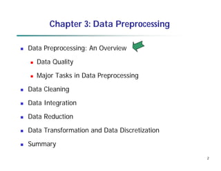
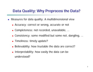
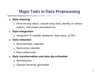
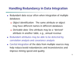
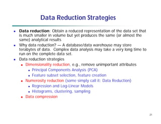
This document provides an overview of data preprocessing techniques. It discusses data quality issues like missing values, noise, and inconsistencies that require cleaning. Major tasks in preprocessing include data cleaning, integration, reduction, and transformation. Data cleaning techniques are described for handling incomplete, noisy, and inconsistent data. Methods for data integration, reduction through dimensionality reduction and sampling, and transformation through normalization and discretization are also summarized.

1. 1
Data Mining:
Concepts and Techniques
(3rd ed.)
— Chapter 3 —
Jiawei Han, Micheline Kamber, and Jian Pei
University of Illinois at Urbana-Champaign &
Simon Fraser University
©2011 Han, Kamber & Pei. All rights reserved.

2. 2
2
Chapter 3: Data Preprocessing
 Data Preprocessing: An Overview
 Data Quality
 Major Tasks in Data Preprocessing
 Data Cleaning
 Data Integration
 Data Reduction
 Data Transformation and Data Discretization
 Summary

3. 3
Data Quality: Why Preprocess the Data?
 Measures for data quality: A multidimensional view
 Accuracy: correct or wrong, accurate or not
 Completeness: not recorded, unavailable, …
 Consistency: some modified but some not, dangling, …
 Timeliness: timely update?
 Believability: how trustable the data are correct?
 Interpretability: how easily the data can be
understood?

4. 4
Major Tasks in Data Preprocessing
 Data cleaning
 Fill in missing values, smooth noisy data, identify or remove
outliers, and resolve inconsistencies
 Data integration
 Integration of multiple databases, data cubes, or files
 Data reduction
 Dimensionality reduction
 Numerosity reduction
 Data compression
 Data transformation and data discretization
 Normalization
 Concept hierarchy generation

5. 5
5
Chapter 3: Data Preprocessing
 Data Preprocessing: An Overview
 Data Quality
 Major Tasks in Data Preprocessing
 Data Cleaning
 Data Integration
 Data Reduction
 Data Transformation and Data Discretization
 Summary

6. 6
Data Cleaning
 Data in the Real World Is Dirty: Lots of potentially incorrect data,
e.g., instrument faulty, human or computer error, transmission error
 incomplete: lacking attribute values, lacking certain attributes of
interest, or containing only aggregate data
 e.g., Occupation=“ ” (missing data)
 noisy: containing noise, errors, or outliers
 e.g., Salary=“−10” (an error)
 inconsistent: containing discrepancies in codes or names, e.g.,
 Age=“42”, Birthday=“03/07/2010”
 Was rating “1, 2, 3”, now rating “A, B, C”
 discrepancy between duplicate records
 Intentional (e.g., disguised missing data)
 Jan. 1 as everyone’s birthday?

7. 7
Incomplete (Missing) Data
 Data is not always available
 E.g., many tuples have no recorded value for several
attributes, such as customer income in sales data
 Missing data may be due to
 equipment malfunction
 inconsistent with other recorded data and thus deleted
 data not entered due to misunderstanding
 certain data may not be considered important at the
time of entry
 not register history or changes of the data
 Missing data may need to be inferred

8. 8
How to Handle Missing Data?
 Ignore the tuple: usually done when class label is missing
(when doing classification)—not effective when the % of
missing values per attribute varies considerably
 Fill in the missing value manually: tedious + infeasible?
 Fill in it automatically with
 a global constant : e.g., “unknown”, a new class?!
 the attribute mean
 the attribute mean for all samples belonging to the
same class: smarter
 the most probable value: inference-based such as
Bayesian formula or decision tree

9. 9
Noisy Data
 Noise: random error or variance in a measured variable
 Incorrect attribute values may be due to
 faulty data collection instruments
 data entry problems
 data transmission problems
 technology limitation
 inconsistency in naming convention
 Other data problems which require data cleaning
 duplicate records
 incomplete data
 inconsistent data

10. 10
How to Handle Noisy Data?
 Binning
 first sort data and partition into (equal-frequency) bins
 then one can smooth by bin means, smooth by bin
median, smooth by bin boundaries, etc.
 Regression
 smooth by fitting the data into regression functions
 Clustering
 detect and remove outliers
 Combined computer and human inspection
 detect suspicious values and check by human (e.g.,
deal with possible outliers)

11. 11
11
Chapter 3: Data Preprocessing
 Data Preprocessing: An Overview
 Data Quality
 Major Tasks in Data Preprocessing
 Data Cleaning
 Data Integration
 Data Reduction
 Data Transformation and Data Discretization
 Summary

12. 12
12
Data Integration
 Data integration:
 Combines data from multiple sources into a coherent store
 Schema integration: e.g., A.cust-id  B.cust-#
 Integrate metadata from different sources
 Entity identification problem:
 Identify real world entities from multiple data sources, e.g., Bill
Clinton = William Clinton
 Detecting and resolving data value conflicts
 For the same real world entity, attribute values from different
sources are different
 Possible reasons: different representations, different scales, e.g.,
meter v.s. kilometer

13. 13
13
Handling Redundancy in Data Integration
 Redundant data occur often when integration of multiple
databases
 Object identification: The same attribute or object
may have different names in different databases
 Derivable data: One attribute may be a “derived”
attribute in another table, e.g., annual revenue
 Redundant attributes may be able to be detected by
correlation analysis and covariance analysis
 Careful integration of the data from multiple sources may
help reduce/avoid redundancies and inconsistencies and
improve mining speed and quality

14. 14
Correlation Analysis (Nominal Data)
 Χ2 (chi-square) test
 The larger the Χ2 value, the more likely the variables are
related
 The cells that contribute the most to the Χ2 value are
those whose actual count is very different from the
expected count
 Correlation does not imply causality
 # of hospitals and # of car-theft in a city are correlated
 Both are causally linked to the third variable: population



Expected
Expected
Observed 2
2 )
(


15. 15
Chi-Square Calculation: An Example
 Χ2 (chi-square) calculation (numbers in parenthesis are
expected counts calculated based on the data distribution
in the two categories)
 It shows that like_science_fiction and play_chess are
correlated in the group
93
.
507
840
)
840
1000
(
360
)
360
200
(
210
)
210
50
(
90
)
90
250
( 2
2
2
2
2










Play chess Not play chess Sum (row)
Like science fiction 250(90) 200(360) 450
Not like science fiction 50(210) 1000(840) 1050
Sum(col.) 300 1200 1500

16. 16
Correlation Analysis (Numeric Data)
 Correlation coefficient (also called Pearson’s product
moment coefficient)
where n is the number of tuples, and are the respective
means of A and B, σA and σB are the respective standard deviation
of A and B, and Σ(aibi) is the sum of the AB cross-product.
 If rA,B > 0, A and B are positively correlated (A’s values
increase as B’s). The higher, the stronger correlation.
 rA,B = 0: independent; rAB < 0: negatively correlated
B
A
n
i i
i
B
A
n
i i
i
B
A
n
B
A
n
b
a
n
B
b
A
a
r





 





 1
1
,
)
(
)
)(
(
A B

17. 17
Visually Evaluating Correlation
Scatter plots
showing the
similarity from
–1 to 1.

18. 18
Covariance (Numeric Data)
 Covariance is similar to correlation
where n is the number of tuples, and are the respective mean or
expected values of A and B, σA and σB are the respective standard
deviation of A and B.
 Positive covariance: If CovA,B > 0, then A and B both tend to be larger
than their expected values.
 Negative covariance: If CovA,B < 0 then if A is larger than its expected
value, B is likely to be smaller than its expected value.
 Independence: CovA,B = 0 but the converse is not true:
 Some pairs of random variables may have a covariance of 0 but are not
independent. Only under some additional assumptions (e.g., the data follow
multivariate normal distributions) does a covariance of 0 imply independence
A B
Correlation coefficient:

19. Co-Variance: An Example
 It can be simplified in computation as
 Suppose two stocks A and B have the following values in one week:
(2, 5), (3, 8), (5, 10), (4, 11), (6, 14).
 Question: If the stocks are affected by the same industry trends, will
their prices rise or fall together?
 E(A) = (2 + 3 + 5 + 4 + 6)/ 5 = 20/5 = 4
 E(B) = (5 + 8 + 10 + 11 + 14) /5 = 48/5 = 9.6
 Cov(A,B) = (2×5+3×8+5×10+4×11+6×14)/5 − 4 × 9.6 = 4
 Thus, A and B rise together since Cov(A, B) > 0.

20. 20
20
Chapter 3: Data Preprocessing
 Data Preprocessing: An Overview
 Data Quality
 Major Tasks in Data Preprocessing
 Data Cleaning
 Data Integration
 Data Reduction
 Data Transformation and Data Discretization
 Summary

21. 21
Data Reduction Strategies
 Data reduction: Obtain a reduced representation of the data set that
is much smaller in volume but yet produces the same (or almost the
same) analytical results
 Why data reduction? — A database/data warehouse may store
terabytes of data. Complex data analysis may take a very long time to
run on the complete data set.
 Data reduction strategies
 Dimensionality reduction, e.g., remove unimportant attributes
 Principal Components Analysis (PCA)
 Feature subset selection, feature creation
 Numerosity reduction (some simply call it: Data Reduction)
 Regression and Log-Linear Models
 Histograms, clustering, sampling
 Data compression

22. 22
Data Reduction 1: Dimensionality Reduction
 Curse of dimensionality
 When dimensionality increases, data becomes increasingly sparse
 Density and distance between points, which is critical to clustering, outlier
analysis, becomes less meaningful
 The possible combinations of subspaces will grow exponentially
 Dimensionality reduction
 Avoid the curse of dimensionality
 Help eliminate irrelevant features and reduce noise
 Reduce time and space required in data mining
 Dimensionality reduction techniques
 Principal Component Analysis
 Supervised and nonlinear techniques (e.g., feature selection)

23. 23
Attribute Creation (Feature Generation)
 Create new attributes (features) that can capture the
important information in a data set more effectively than
the original ones
 Three general methodologies
 Attribute extraction
 Domain-specific
 Mapping data to new space (see: data reduction)
 Using kernel functions
 Combining features
 Data discretization

24. 24
Clustering
 Partition data set into clusters based on similarity, and
store cluster representation (e.g., centroid and diameter)
only
 Can have hierarchical clustering and be stored in multi-
dimensional index tree structures
 There are many choices of clustering definitions and
clustering algorithms

25. 25
Sampling
 Sampling: obtaining a small sample s to represent the
whole data set N
 Allow a mining algorithm to run in complexity that is
potentially sub-linear to the size of the data
 Key principle: Choose a representative subset of the data
 Simple random sampling may have very poor
performance in the presence of skew
 Develop adaptive sampling methods, e.g., stratified
sampling

26. 26
Types of Sampling
 Simple random sampling
 There is an equal probability of selecting any particular
item
 Sampling without replacement
 Once an object is selected, it is removed from the
population
 Sampling with replacement
 A selected object is not removed from the population
 Stratified sampling:
 Partition the data set, and draw samples from each
partition (proportionally, i.e., approximately the same
percentage of the data)
 Used in conjunction with skewed data

27. 27
Sampling: With or without Replacement
Raw Data

28. 28
Sampling: Cluster or Stratified Sampling
Raw Data Cluster/Stratified Sample

29. 29
Data Reduction 3: Data Compression
 String compression
 There are extensive theories and well-tuned algorithms
 Typically lossless, but only limited manipulation is
possible without expansion
 Audio/video compression
 Typically lossy compression, with progressive refinement
 Sometimes small fragments of signal can be
reconstructed without reconstructing the whole
 Dimensionality and numerosity reduction may also be
considered as forms of data compression

30. 30
Data Compression
Original Data Compressed
Data
lossless
Original Data
Approximated

31. 31
Chapter 3: Data Preprocessing
 Data Preprocessing: An Overview
 Data Quality
 Major Tasks in Data Preprocessing
 Data Cleaning
 Data Integration
 Data Reduction
 Data Transformation and Data Discretization
 Summary

32. 32
Data Transformation
 A function that maps the entire set of values of a given attribute to a
new set of replacement values s.t. each old value can be identified
with one of the new values
 Methods
 Smoothing: Remove noise from data
 Attribute/feature construction
 New attributes constructed from the given ones
 Aggregation: Summarization, data cube construction
 Normalization: Scaled to fall within a smaller, specified range
 min-max normalization
 z-score normalization
 normalization by decimal scaling
 Discretization: Concept hierarchy climbing

33. 33
Normalization
 Min-max normalization: to [new_minA, new_maxA]
 Ex. Let income range $12,000 to $98,000 normalized to [0.0,
1.0]. Then $73,000 is mapped to
 Z-score normalization (μ: mean, σ: standard deviation):
 Ex. Let μ = 54,000, σ = 16,000. Then
 Normalization by decimal scaling
716
.
0
0
)
0
0
.
1
(
000
,
12
000
,
98
000
,
12
600
,
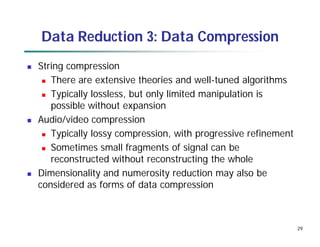
73





A
A
A
A
A
A
min
new
min
new
max
new
min
max
min
v
v _
)
_
_
(
' 




A
A
v
v




'
j
v
v
10
' Where j is the smallest integer such that Max(|ν’|) < 1
225
.
1
000
,
16
000
,
54
600
,
73



34. 34
Discretization
 Three types of attributes
 Nominal—values from an unordered set, e.g., color, profession
 Ordinal—values from an ordered set, e.g., military or academic
rank
 Numeric—real numbers, e.g., integer or real numbers
 Discretization: Divide the range of a continuous attribute into intervals
 Interval labels can then be used to replace actual data values
 Reduce data size by discretization
 Supervised vs. unsupervised
 Split (top-down) vs. merge (bottom-up)
 Discretization can be performed recursively on an attribute
 Prepare for further analysis, e.g., classification

35. 35
Data Discretization Methods
 Typical methods: All the methods can be applied recursively
 Binning
 Top-down split, unsupervised
 Histogram analysis
 Top-down split, unsupervised
 Clustering analysis (unsupervised, top-down split or
bottom-up merge)
 Decision-tree analysis (supervised, top-down split)
 Correlation (e.g., 2) analysis (unsupervised, bottom-up
merge)

36. 36
Simple Discretization: Binning
 Equal-width (distance) partitioning
 Divides the range into N intervals of equal size: uniform grid
 if A and B are the lowest and highest values of the attribute, the
width of intervals will be: W = (B –A)/N.
 The most straightforward, but outliers may dominate presentation
 Skewed data is not handled well
 Equal-depth (frequency) partitioning
 Divides the range into N intervals, each containing approximately
same number of samples
 Good data scaling
 Managing categorical attributes can be tricky

37. 37
Binning Methods for Data Smoothing
 Sorted data for price (in dollars): 4, 8, 9, 15, 21, 21, 24, 25, 26,
28, 29, 34
* Partition into equal-frequency (equi-depth) bins:
- Bin 1: 4, 8, 9, 15
- Bin 2: 21, 21, 24, 25
- Bin 3: 26, 28, 29, 34
* Smoothing by bin means:
- Bin 1: 9, 9, 9, 9
- Bin 2: 23, 23, 23, 23
- Bin 3: 29, 29, 29, 29
* Smoothing by bin boundaries:
- Bin 1: 4, 4, 4, 15
- Bin 2: 21, 21, 25, 25
- Bin 3: 26, 26, 26, 34

38. 38
Discretization by Classification &
Correlation Analysis
 Classification (e.g., decision tree analysis)
 Supervised: Given class labels, e.g., cancerous vs. benign
 Using entropy to determine split point (discretization point)
 Top-down, recursive split
 Details to be covered in Chapter 7
 Correlation analysis (e.g., Chi-merge: χ2-based discretization)
 Supervised: use class information
 Bottom-up merge: find the best neighboring intervals (those
having similar distributions of classes, i.e., low χ2 values) to merge
 Merge performed recursively, until a predefined stopping condition

39. 39
Chapter 3: Data Preprocessing
 Data Preprocessing: An Overview
 Data Quality
 Major Tasks in Data Preprocessing
 Data Cleaning
 Data Integration
 Data Reduction
 Data Transformation and Data Discretization
 Summary

40. 40
Summary
 Data quality: accuracy, completeness, consistency, timeliness,
believability, interpretability
 Data cleaning: e.g. missing/noisy values, outliers
 Data integration from multiple sources:
 Entity identification problem
 Remove redundancies
 Detect inconsistencies
 Data reduction
 Dimensionality reduction
 Numerosity reduction
 Data compression
 Data transformation and data discretization
 Normalization
 Concept hierarchy generation