Data Mining Lecture_5.pptx

DATA MINING
LECTURE 5
Similarity and Distance
Sketching, Locality Sensitive Hashing
Subrata Kumer Paul
Assistant Professor, Dept. of CSE, BAUET
sksubrata96@gmail.com

SIMILARITY AND
DISTANCE
Thanks to:
Tan, Steinbach, and Kumar, “Introduction to Data Mining”
Rajaraman and Ullman, “Mining Massive Datasets”

Similarity and Distance
• For many different problems we need to quantify how
close two objects are.
• Examples:
• For an item bought by a customer, find other similar items
• Group together the customers of site so that similar customers are
shown the same ad.
• Group together web documents so that you can separate the ones
that talk about politics and the ones that talk about sports.
• Find all the near-duplicate mirrored web documents.
• Find credit card transactions that are very different from previous
transactions.
• To solve these problems we need a definition of similarity,
or distance.
• The definition depends on the type of data that we have

Similarity
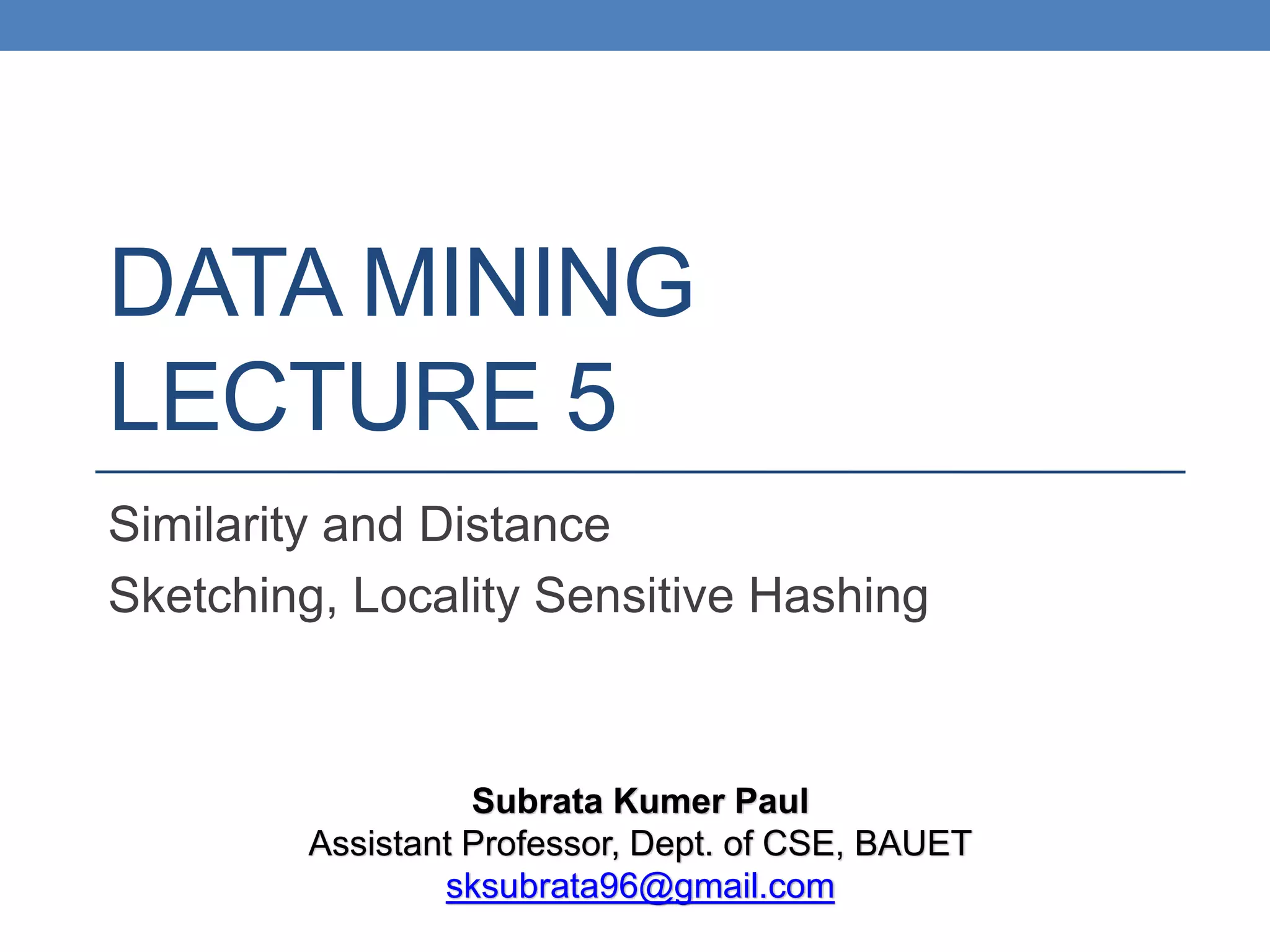
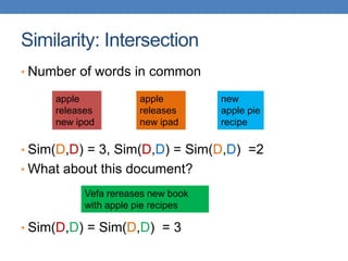
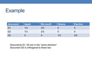
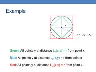
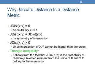
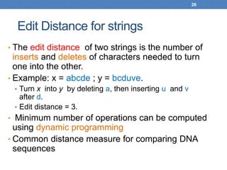
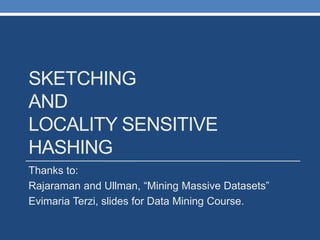
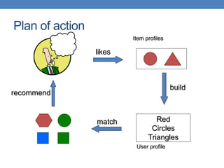
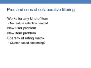
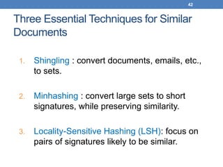
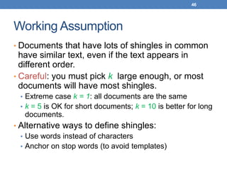
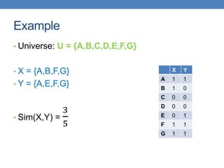
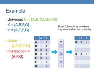
• Numerical measure of how alike two data objects
are.
• A function that maps pairs of objects to real values
• Higher when objects are more alike.
• Often falls in the range [0,1], sometimes in [-1,1]
• Desirable properties for similarity
1. s(p, q) = 1 (or maximum similarity) only if p = q.
(Identity)
2. s(p, q) = s(q, p) for all p and q. (Symmetry)

Similarity between sets
• Consider the following documents
• Which ones are more similar?
• How would you quantify their similarity?
apple
releases
new ipod
apple
releases
new ipad
new
apple pie
recipe

Similarity: Intersection
• Number of words in common
• Sim(D,D) = 3, Sim(D,D) = Sim(D,D) =2
• What about this document?
• Sim(D,D) = Sim(D,D) = 3
apple
releases
new ipod
apple
releases
new ipad
new
apple pie
recipe
Vefa rereases new book
with apple pie recipes

7
Jaccard Similarity
• The Jaccard similarity (Jaccard coefficient) of two sets S1,
S2 is the size of their intersection divided by the size of
their union.
• JSim (C1, C2) = |C1C2| / |C1C2|.
• Extreme behavior:
• Jsim(X,Y) = 1, iff X = Y
• Jsim(X,Y) = 0 iff X,Y have not elements in common
• JSim is symmetric
3 in intersection.
8 in union.
Jaccard similarity
= 3/8

Similarity: Intersection
• Number of words in common
• JSim(D,D) = 3/5
• JSim(D,D) = JSim(D,D) = 2/6
• JSim(D,D) = JSim(D,D) = 3/9
apple
releases
new ipod
apple
releases
new ipad
new
apple pie
recipe
Vefa rereases
new book with
apple pie
recipes

Similarity between vectors
document Apple Microsoft Obama Election
D1 10 20 0 0
D2 30 60 0 0
D2 0 0 10 20
Documents (and sets in general) can also be represented as vectors
How do we measure the similarity of two vectors?
How well are the two vectors aligned?

Example
D1 1/3 2/3 0 0
D2 1/3 2/3 0 0
D2 0 0 1/3 2/3
Documents D1, D2 are in the “same direction”
Document D3 is orthogonal to these two

Cosine Similarity
• Sim(X,Y) = cos(X,Y)
• The cosine of the angle between X and Y
• If the vectors are aligned (correlated) angle is zero degrees and
cos(X,Y)=1
• If the vectors are orthogonal (no common coordinates) angle is 90
degrees and cos(X,Y) = 0
• Cosine is commonly used for comparing documents, where we
assume that the vectors are normalized by the document length.

Cosine Similarity - math
• If d1 and d2 are two vectors, then
cos( d1, d2 ) = (d1  d2) / ||d1|| ||d2|| ,
where  indicates vector dot product and || d || is the length of vector d.
• Example:
d1 = 3 2 0 5 0 0 0 2 0 0
d2 = 1 0 0 0 0 0 0 1 0 2
d1  d2= 3*1 + 2*0 + 0*0 + 5*0 + 0*0 + 0*0 + 0*0 + 2*1 + 0*0 + 0*2 = 5
||d1|| = (3*3+2*2+0*0+5*5+0*0+0*0+0*0+2*2+0*0+0*0)0.5 = (42) 0.5 = 6.481
||d2|| = (1*1+0*0+0*0+0*0+0*0+0*0+0*0+1*1+0*0+2*2) 0.5 = (6) 0.5 = 2.245
cos( d1, d2 ) = .3150

Similarity between vectors
D1 10 20 0 0
D2 30 60 0 0
D2 0 0 10 20
cos(D1,D2) = 1
cos(D1,D3) = cos(D2,D3) = 0

Distance
• Numerical measure of how different two data
objects are
• A function that maps pairs of objects to real values
• Lower when objects are more alike
• Minimum distance is 0, when comparing an
object with itself.
• Upper limit varies

Distance Metric
• A distance function d is a distance metric if it is a
function from pairs of objects to real numbers
such that:
1. d(x,y) > 0. (non-negativity)
2. d(x,y) = 0 iff x = y. (identity)
3. d(x,y) = d(y,x). (symmetry)
4. d(x,y) < d(x,z) + d(z,y) (triangle inequality ).

Triangle Inequality
• Triangle inequality guarantees that the distance
function is well-behaved.
• The direct connection is the shortest distance
• It is useful also for proving properties about the
data
• For example, suppose I want to find an object that
minimizes the sum of distances to all points in my
dataset
• If I select the best point from my dataset, the sum of
distances I get is at most twice that of the optimal point.

Distances for real vectors
• Vectors 𝑥 = 𝑥1, … , 𝑥𝑑 and 𝑦 = (𝑦1, … , 𝑦𝑑)
• Lp norms or Minkowski distance:
𝐿𝑝 𝑥, 𝑦 = 𝑥1 − 𝑦1
𝑝
+ ⋯ + 𝑥𝑑 − 𝑦𝑑
𝑝 1
𝑝
• L2 norm: Euclidean distance:
𝐿2 𝑥, 𝑦 = 𝑥1 − 𝑦1
2 + ⋯ + 𝑥𝑑 − 𝑦𝑑
2
• L1 norm: Manhattan distance:
𝐿1 𝑥, 𝑦 = 𝑥1 − 𝑦1 + ⋯ + |𝑥𝑑 − 𝑦𝑑|
• L∞ norm:
𝐿∞ 𝑥, 𝑦 = max 𝑥1 − 𝑦1 , … , |𝑥𝑑 − 𝑦𝑑|
• The limit of Lp as p goes to infinity.
Lp norms are known to be distance metrics

18
Example of Distances
x = (5,5)
y = (9,8)
L2-norm:
𝑑𝑖𝑠𝑡(𝑥, 𝑦) = 42 + 32 = 5
L1-norm:
𝑑𝑖𝑠𝑡(𝑥, 𝑦) = 4 + 3 = 7
4
3
5
L∞-norm:
𝑑𝑖𝑠𝑡(𝑥, 𝑦) = max 3,4 = 4

Example
𝑥 = (𝑥1, … , 𝑥𝑛)
r
Green: All points y at distance L1(x,y) = r from point x
Blue: All points y at distance L2(x,y) = r from point x
Red: All points y at distance L∞(x,y) = r from point x

Lp distances for sets
• We can apply all the Lp distances to the cases of
sets of attributes, with or without counts, if we
represent the sets as vectors
• E.g., a transaction is a 0/1 vector
• E.g., a document is a vector of counts.

Similarities into distances
• Jaccard distance:
𝐽𝐷𝑖𝑠𝑡(𝑋, 𝑌) = 1 – 𝐽𝑆𝑖𝑚(𝑋, 𝑌)
• Jaccard Distance is a metric
• Cosine distance:
𝐷𝑖𝑠𝑡(𝑋, 𝑌) = 1 − cos(𝑋, 𝑌)
• Cosine distance is a metric

22
Why Jaccard Distance Is a Distance
Metric
• JDist(x,x) = 0
• since JSim(x,x) = 1
• JDist(x,y) = JDist(y,x)
• by symmetry of intersection
• JDist(x,y) > 0
• since intersection of X,Y cannot be bigger than the union.
• Triangle inequality:
• Follows from the fact that JSim(X,Y) is the probability of
randomly selected element from the union of X and Y to
belong to the intersection

23
Hamming Distance
• Hamming distance is the number of positions in
which bit-vectors differ.
• Example: p1 = 10101
p2 = 10011.
• d(p1, p2) = 2 because the bit-vectors differ in the 3rd and 4th
positions.
• The L1 norm for the binary vectors
• Hamming distance between two vectors of
categorical attributes is the number of positions in
which they differ.
• Example: x = (married, low income, cheat),
y = (single, low income, not cheat)
• d(x,y) = 2

24
Why Hamming Distance Is a Distance
Metric
• d(x,x) = 0 since no positions differ.
• d(x,y) = d(y,x) by symmetry of “different from.”
• d(x,y) > 0 since strings cannot differ in a negative
number of positions.
• Triangle inequality: changing x to z and then to y
is one way to change x to y.
• For binary vectors if follows from the fact that L1
norm is a metric

Distance between strings
• How do we define similarity between strings?
• Important for recognizing and correcting typing
errors and analyzing DNA sequences.
weird wierd
intelligent unintelligent
Athena Athina

26
Edit Distance for strings
• The edit distance of two strings is the number of
inserts and deletes of characters needed to turn
one into the other.
• Example: x = abcde ; y = bcduve.
• Turn x into y by deleting a, then inserting u and v
after d.
• Edit distance = 3.
• Minimum number of operations can be computed
using dynamic programming
• Common distance measure for comparing DNA
sequences

27
Why Edit Distance Is a Distance Metric
• d(x,x) = 0 because 0 edits suffice.
• d(x,y) = d(y,x) because insert/delete are
inverses of each other.
• d(x,y) > 0: no notion of negative edits.
• Triangle inequality: changing x to z and then
to y is one way to change x to y. The
minimum is no more than that

28
Variant Edit Distances
• Allow insert, delete, and mutate.
• Change one character into another.
• Minimum number of inserts, deletes, and
mutates also forms a distance measure.
• Same for any set of operations on strings.
• Example: substring reversal or block transposition OK
for DNA sequences
• Example: character transposition is used for spelling

Distances between distributions
• We can view a document as a distribution over the words
• KL-divergence (Kullback-Leibler) for distributions P,Q
𝐷𝐾𝐿 𝑃 𝑄 =
𝑥
𝑝 𝑥 log
𝑝(𝑥)
𝑞(𝑥)
• KL-divergence is asymmetric. We can make it symmetric by
taking the average of both sides
• JS-divergence (Jensen-Shannon)
𝐽𝑆 𝑃, 𝑄 =
1
2
𝐷𝐾𝐿 𝑃 𝑄 +
1
2
𝐷𝐾𝐿 𝑄 𝑃
D1 0.35 0.5 0.1 0.05
D2 0.4 0.4 0.1 0.1
D2 0.05 0.05 0.6 0.3

SKETCHING
AND
LOCALITY SENSITIVE
HASHING
Thanks to:
Rajaraman and Ullman, “Mining Massive Datasets”
Evimaria Terzi, slides for Data Mining Course.

Why is similarity important?
• We saw many definitions of similarity and
distance
• How do we make use of similarity in practice?
• What issues do we have to deal with?

An important problem
• Recommendation systems
• When a user buys an item (initially books) we want to
recommend other items that the user may like
• When a user rates a movie, we want to recommend
movies that the user may like
• When a user likes a song, we want to recommend other
songs that they may like
• A big success of data mining
• Exploits the long tail

Recommendation Systems
• Content-based:
• Represent the items into a feature space and
recommend items to customer C similar to previous
items rated highly by C
• Movie recommendations: recommend movies with same
actor(s), director, genre, …
• Websites, blogs, news: recommend other sites with “similar”
content

Plan of action
likes
Item profiles
Red
Circles
Triangles
User profile
match
recommend
build

Limitations of content-based approach
• Finding the appropriate features
• e.g., images, movies, music
• Overspecialization
• Never recommends items outside user’s content profile
• People might have multiple interests
• Recommendations for new users
• How to build a profile?

Recommendation Systems (II)
• Collaborative Filtering (user –user)
• Consider user c
• Find set D of other users whose ratings are
“similar” to c’s ratings
• Estimate user’s ratings based on ratings of
users in D

Recommendation Systems (III)
• Collaborative filtering (item-item)
• For item s, find other similar items
• Estimate rating for item based on ratings for
similar items
• Can use same similarity metrics and prediction
functions as in user-user model
• In practice, it has been observed that item-
item often works better than user-user

Pros and cons of collaborative filtering
• Works for any kind of item
• No feature selection needed
• New user problem
• New item problem
• Sparsity of rating matrix
• Cluster-based smoothing?

Another important problem
• Find duplicate and near-duplicate documents
from a web crawl.
• Why is it important:
• Identify mirrored web pages, and avoid indexing them,
or serving them multiple times
• Find replicated news stories and cluster them under a
single story.
• Identify plagiarism
• What if we wanted exact duplicates?

Finding similar items
• Both the problems we described have a common
component
• We need a quick way to find highly similar items to a
query item
• OR, we need a method for finding all pairs of items that
are highly similar.
• Also known as the Nearest Neighbor problem, or
the All Nearest Neighbors problem
• We will examine it for the case of near-duplicate
web documents.

Main issues
• What is the right representation of the document
when we check for similarity?
• E.g., representing a document as a set of characters
will not do (why?)
• When we have billions of documents, keeping the
full text in memory is not an option.
• We need to find a shorter representation
• How do we do pairwise comparisons of billions of
documents?
• If exact match was the issue it would be ok, can we
replicate this idea?

42
Three Essential Techniques for Similar
Documents
1. Shingling : convert documents, emails, etc.,
to sets.
2. Minhashing : convert large sets to short
signatures, while preserving similarity.
3. Locality-Sensitive Hashing (LSH): focus on
pairs of signatures likely to be similar.

43
The Big Picture
Docu-
ment
The set
of strings
of length k
that appear
in the doc-
ument
Signatures :
short integer
vectors that
represent the
sets, and
reflect their
similarity
Locality-
sensitive
Hashing
Candidate
pairs :
those pairs
of signatures
that we need
to test for
similarity.

44
Shingles
• A k -shingle (or k -gram) for a document is a
sequence of k characters that appears in the
document.
• Example: document = abcab. k=2
• Set of 2-shingles = {ab, bc, ca}.
• Option: regard shingles as a bag, and count ab twice.
• Represent a document by its set of k-shingles.

Shingling
• Shingle: a sequence of k contiguous characters
a rose is a rose is a rose
a rose is
rose is a
rose is a
ose is a r
se is a ro
e is a ros
is a rose
is a rose
s a rose i
a rose is
a rose is

46
Working Assumption
• Documents that have lots of shingles in common
have similar text, even if the text appears in
different order.
• Careful: you must pick k large enough, or most
documents will have most shingles.
• Extreme case k = 1: all documents are the same
• k = 5 is OK for short documents; k = 10 is better for long
documents.
• Alternative ways to define shingles:
• Use words instead of characters
• Anchor on stop words (to avoid templates)

47
Shingles: Compression Option
• To compress long shingles, we can hash them
to (say) 4 bytes.
• Represent a doc by the set of hash values of
its k-shingles.
• From now on we will assume that shingles are
integers
• Collisions are possible, but very rare

Fingerprinting
• Hash shingles to 64-bit integers
a rose is
rose is a
rose is a
ose is a r
se is a ro
e is a ros
is a rose
is a rose
s a rose i
a rose is
1111
2222
3333
4444
5555
6666
7777
8888
9999
0000
Set of Shingles Set of 64-bit integers
Hash function
(Rabin’s fingerprints)

49
Basic Data Model: Sets
• Document: A document is represented as a set
shingles (more accurately, hashes of shingles)
• Document similarity: Jaccard similarity of the sets of
shingles.
• Common shingles over the union of shingles
• Sim (C1, C2) = |C1C2|/|C1C2|.
• Although we use the documents as our driving
example the techniques we will describe apply to any
kind of sets.
• E.g., similar customers or items.

Signatures
• Problem: shingle sets are too large to be kept in memory.
• Key idea: “hash” each set S to a small signature Sig (S),
such that:
1. Sig (S) is small enough that we can fit a signature in main
memory for each set.
2. Sim (S1, S2) is (almost) the same as the “similarity” of Sig (S1)
and Sig (S2). (signature preserves similarity).
• Warning: This method can produce false negatives, and
false positives (if an additional check is not made).
• False negatives: Similar items deemed as non-similar
• False positives: Non-similar items deemed as similar

51
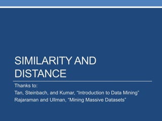
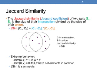
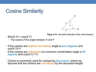
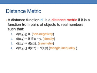
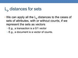
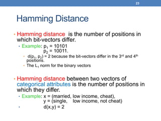
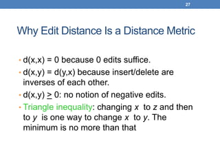
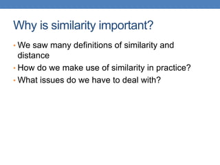
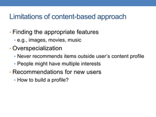
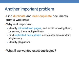
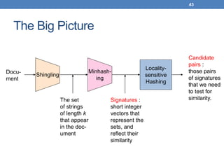
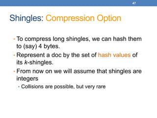
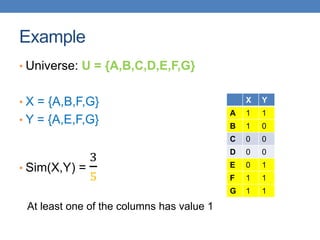
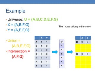
From Sets to Boolean Matrices
• Represent the data as a boolean matrix M
• Rows = the universe of all possible set elements
• In our case, shingle fingerprints take values in [0…264-1]
• Columns = the sets
• In our case, documents, sets of shingle fingerprints
• M(r,S) = 1 in row r and column S if and only if r is a
member of S.
• Typical matrix is sparse.
• We do not really materialize the matrix

Example
• Universe: U = {A,B,C,D,E,F,G}
• X = {A,B,F,G}
• Y = {A,E,F,G}
• Sim(X,Y) =
3
5
X Y
A 1 1
B 1 0
C 0 0
D 0 0
E 0 1
F 1 1
G 1 1

Example
• X = {A,B,F,G}
• Y = {A,E,F,G}
• Sim(X,Y) =
3
5
X Y
A 1 1
B 1 0
C 0 0
D 0 0
E 0 1
F 1 1
G 1 1
At least one of the columns has value 1

Example
• X = {A,B,F,G}
• Y = {A,E,F,G}
• Sim(X,Y) =
3
5
X Y
A 1 1
B 1 0
C 0 0
D 0 0
E 0 1
F 1 1
G 1 1
Both columns have value 1

55
Minhashing
• Pick a random permutation of the rows (the
universe U).
• Define “hash” function for set S
• h(S) = the index of the first row (in the permuted order)
in which column S has 1.
• OR
• h(S) = the index of the first element of S in the permuted
order.
• Use k (e.g., k = 100) independent random
permutations to create a signature.

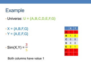
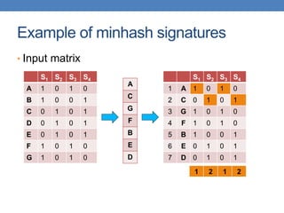
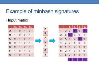
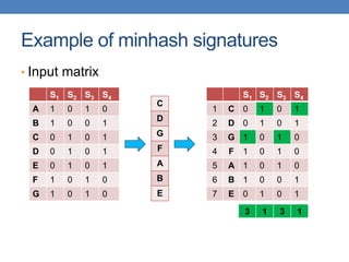
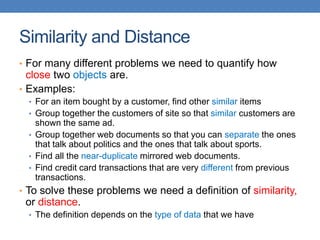
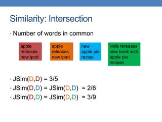
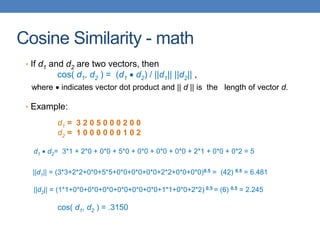
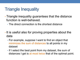
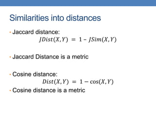
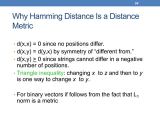
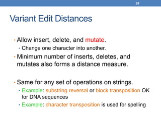
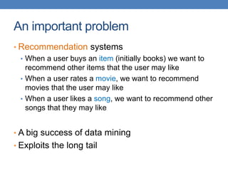
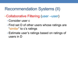
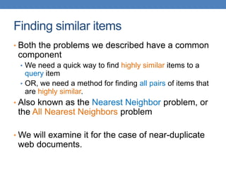
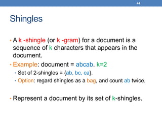
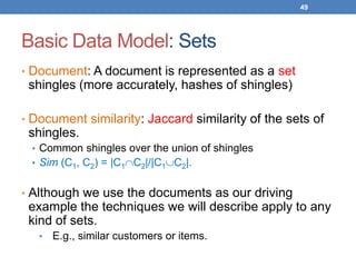
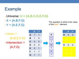
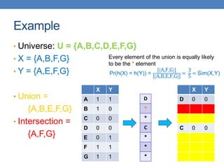
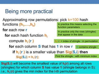
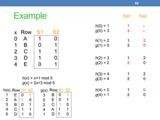
Example of minhash signatures
• Input matrix
S1 S2 S3 S4
A 1 0 1 0
B 1 0 0 1
C 0 1 0 1
D 0 1 0 1
E 0 1 0 1
F 1 0 1 0
G 1 0 1 0
A
C
G
F
B
E
D
S1 S2 S3 S4
1 A 1 0 1 0
2 C 0 1 0 1
3 G 1 0 1 0
4 F 1 0 1 0
5 B 1 0 0 1
6 E 0 1 0 1
7 D 0 1 0 1
1 2 1 2

• Input matrix
S1 S2 S3 S4
A 1 0 1 0
B 1 0 0 1
C 0 1 0 1
D 0 1 0 1
E 0 1 0 1
F 1 0 1 0
G 1 0 1 0
D
B
A
C
F
G
E
S1 S2 S3 S4
1 D 0 1 0 1
2 B 1 0 0 1
3 A 1 0 1 0
4 C 0 1 0 1
5 F 1 0 1 0
6 G 1 0 1 0
7 E 0 1 0 1
2 1 3 1

• Input matrix
S1 S2 S3 S4
A 1 0 1 0
B 1 0 0 1
C 0 1 0 1
D 0 1 0 1
E 0 1 0 1
F 1 0 1 0
G 1 0 1 0
C
D
G
F
A
B
E
S1 S2 S3 S4
1 C 0 1 0 1
2 D 0 1 0 1
3 G 1 0 1 0
4 F 1 0 1 0
5 A 1 0 1 0
6 B 1 0 0 1
7 E 0 1 0 1
3 1 3 1

• Input matrix
S1 S2 S3 S4
A 1 0 1 0
B 1 0 0 1
C 0 1 0 1
D 0 1 0 1
E 0 1 0 1
F 1 0 1 0
G 1 0 1 0
S1 S2 S3 S4
h1 1 2 1 2
h2 2 1 3 1
h3 3 1 3 1
≈
• Sig(S) = vector of hash values
• e.g., Sig(S2) = [2,1,1]
• Sig(S,i) = value of the i-th hash
function for set S
• E.g., Sig(S2,3) = 1
Signature matrix

60
Hash function Property
Pr(h(S1) = h(S2)) = Sim(S1,S2)
• where the probability is over all choices of
permutations.
• Why?
• The first row where one of the two sets has value 1
belongs to the union.
• Recall that union contains rows with at least one 1.
• We have equality if both sets have value 1, and this row
belongs to the intersection

Example
• X = {A,B,F,G}
• Y = {A,E,F,G}
• Union =
{A,B,E,F,G}
• Intersection =
{A,F,G}
X Y
A 1 1
B 1 0
C 0 0
D 0 0
E 0 1
F 1 1
G 1 1
D
*
*
C
*
*
*
X Y
D 0 0
C 0 0
Rows C,D could be anywhere
they do not affect the probability

Example
• X = {A,B,F,G}
• Y = {A,E,F,G}
• Union =
{A,B,E,F,G}
• Intersection =
{A,F,G}
X Y
A 1 1
B 1 0
C 0 0
D 0 0
E 0 1
F 1 1
G 1 1
D
*
*
C
*
*
*
X Y
D 0 0
C 0 0
The * rows belong to the union

Example
• X = {A,B,F,G}
• Y = {A,E,F,G}
• Union =
{A,B,E,F,G}
• Intersection =
{A,F,G}
X Y
A 1 1
B 1 0
C 0 0
D 0 0
E 0 1
F 1 1
G 1 1
D
*
*
C
*
*
*
X Y
D 0 0
C 0 0
The question is what is the value
of the first * element

Example
• X = {A,B,F,G}
• Y = {A,E,F,G}
• Union =
{A,B,E,F,G}
• Intersection =
{A,F,G}
X Y
A 1 1
B 1 0
C 0 0
D 0 0
E 0 1
F 1 1
G 1 1
D
*
*
C
*
*
*
X Y
D 0 0
C 0 0
If it belongs to the intersection
then h(X) = h(Y)

Example
• X = {A,B,F,G}
• Y = {A,E,F,G}
• Union =
{A,B,E,F,G}
• Intersection =
{A,F,G}
X Y
A 1 1
B 1 0
C 0 0
D 0 0
E 0 1
F 1 1
G 1 1
D
*
*
C
*
*
*
X Y
D 0 0
C 0 0
Every element of the union is equally likely
to be the * element
Pr(h(X) = h(Y)) =
| A,F,G |
| A,B,E,F,G |
=
3
5
= Sim(X,Y)

Zero similarity is preserved
High similarity is well approximated
66
Similarity for Signatures
• The similarity of signatures is the fraction of the
hash functions in which they agree.
• With multiple signatures we get a good
approximation
S1 S2 S3 S4
A 1 0 1 0
B 1 0 0 1
C 0 1 0 1
D 0 1 0 1
E 0 1 0 1
F 1 0 1 0
G 1 0 1 0
S1 S2 S3 S4
1 2 1 2
2 1 3 1
3 1 3 1
≈
Actual Sig
(S1, S2) 0 0
(S1, S3) 3/5 2/3
(S1, S4) 1/7 0
(S2, S3) 0 0
(S2, S4) 3/4 1
(S3, S4) 0 0
Signature matrix

Is it now feasible?
• Assume a billion rows
• Hard to pick a random permutation of 1…billion
• Even representing a random permutation
requires 1 billion entries!!!
• How about accessing rows in permuted order?
• 

Being more practical
Approximating row permutations: pick k=100 hash
functions (h1,…,hk)
for each row r
for each hash function hi
compute hi (r )
for each column S that has 1 in row r
if hi (r ) is a smaller value than Sig(S,i) then
Sig(S,i) = hi (r);
Sig(S,i) will become the smallest value of hi(r) among all rows
(shingles) for which column S has value 1 (shingle belongs in S);
i.e., hi (r) gives the min index for the i-th permutation
In practice this means selecting the
function parameters
In practice only the rows (shingles)
that appear in the data
hi (r) = index of shingle r in permutation
S contains shingle r
Find the shingle r with minimum index

69
Example
Row S1 S2
A 1 0
B 0 1
C 1 1
D 1 0
E 0 1
h(x) = x+1 mod 5
g(x) = 2x+3 mod 5
h(0) = 1 1 -
g(0) = 3 3 -
h(1) = 2 1 2
g(1) = 0 3 0
h(2) = 3 1 2
g(2) = 2 2 0
h(3) = 4 1 2
g(3) = 4 2 0
h(4) = 0 1 0
g(4) = 1 2 0
Sig1 Sig2
Row S1 S2
E 0 1
A 1 0
B 0 1
C 1 1
D 1 0
Row S1 S2
B 0 1
E 0 1
C 1 0
A 1 1
D 1 0
x
0
1
2
3
4
h(x)
1
2
3
4
0
g(x)
3
0
2
4
1

70
Implementation – (4)
• Often, data is given by column, not row.
• E.g., columns = documents, rows = shingles.
• If so, sort matrix once so it is by row.
• And always compute hi (r ) only once for each
row.

Data Mining Lecture_5.pptx

Recommended

Recommended

More Related Content

Similar to Data Mining Lecture_5.pptx

Similar to Data Mining Lecture_5.pptx (20)

More from Subrata Kumer Paul

More from Subrata Kumer Paul (20)

Recently uploaded

Recently uploaded (20)

Data Mining Lecture_5.pptx