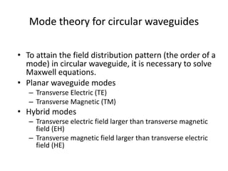
Downloaded 205 times


![Full width at half power (FWHP)
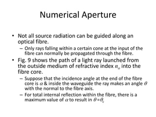
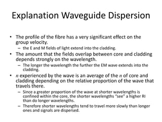
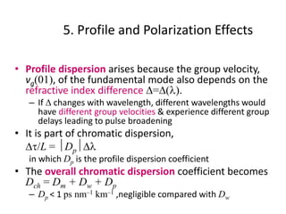
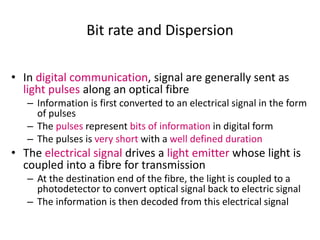
• If a light pulse is fed into the fibre, the output pulse will be
delayed by the transit time t.
• Due to various dispersion mechanism, there will be a spread Dt
in the arrival times of different guided waves.
– The dispersion is measured between half-power points & is called full
width at half-power (FWHP) or full width at half-maximum (FWHM), Dt
= Dt½.
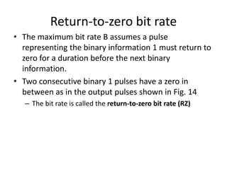
• To clearly distinguish between two consecutive output pulses (no
intersymbol interference), the time-separate from peak to peak
is at least 2Dt½
– So we can only feed in pulses at every 2Dt½ seconds
– Thus the maximum bit rate B is roughly 1/(2Dt½).
B 0.5/(Dt½). [10]](https://image.slidesharecdn.com/chapter2b-140705120853-phpapp02/85/Chapter-2b-40-320.jpg)
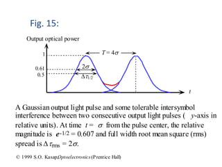
![Analysis for RZ transmission
• For a more rigorous analysis, the temporal shape of
signal & the criterion for discerning the information
should be known.
• For a Gaussian output light pulse, tolerable
interference between two consecutive light output
pulses is 4s between their peaks
• Thus, the bit rate should be B 0.25/s
• Given s = 0.425Dt½ , B = 0.59/Dt½ .
– This is ~18% greater than the intuitive estimation in eqn[10]](https://image.slidesharecdn.com/chapter2b-140705120853-phpapp02/85/Chapter-2b-44-320.jpg)
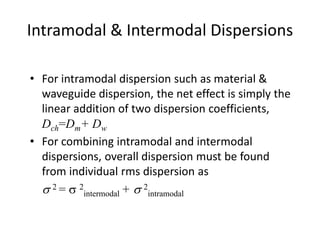

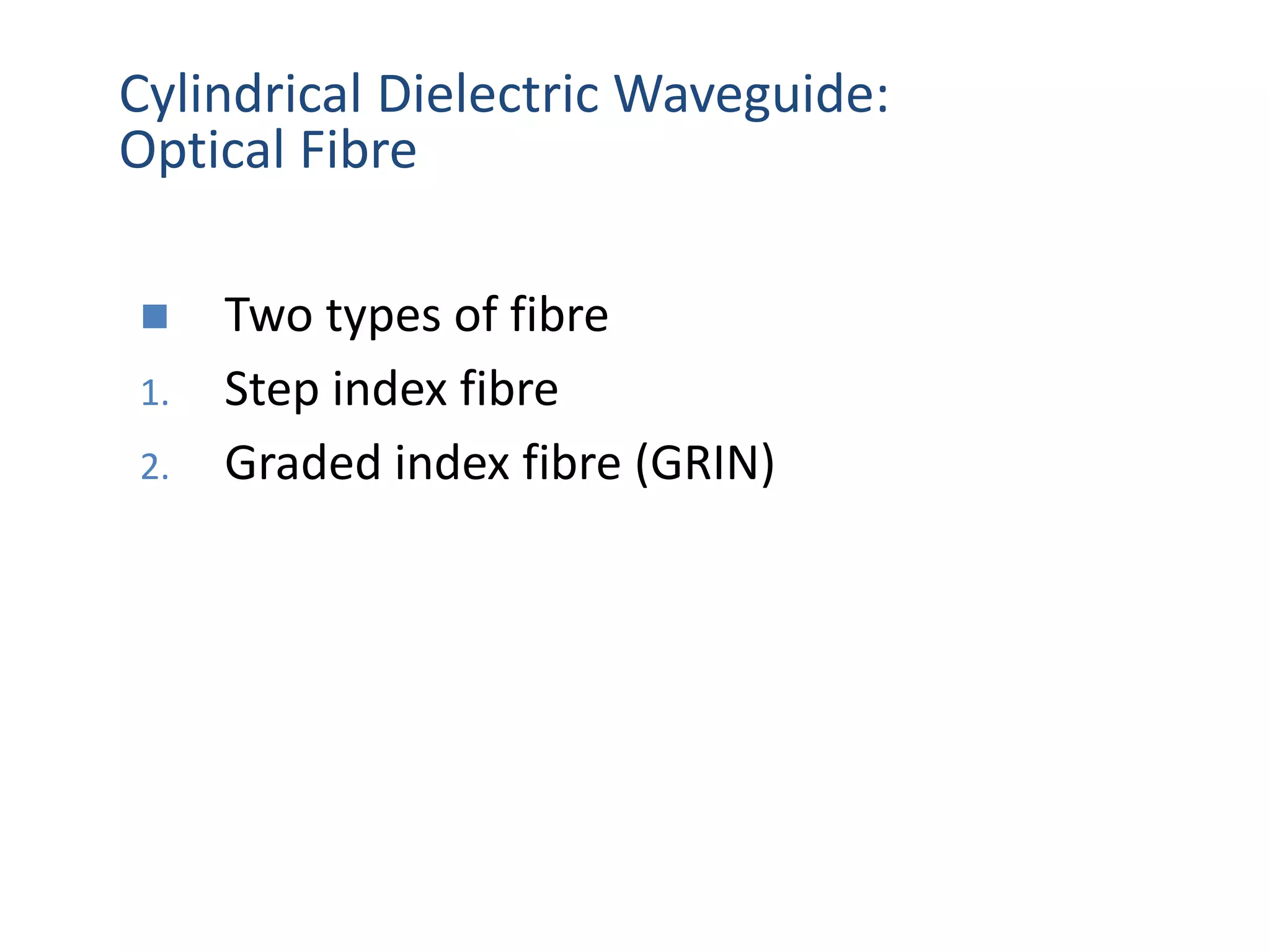
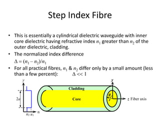
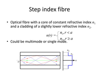
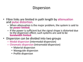
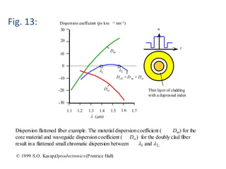
1. The document discusses optical fibers, specifically step index fibers. It describes step index fibers as having a core with a constant refractive index n1 surrounded by a cladding with a slightly lower refractive index n2. 2. It discusses several factors that determine the number of propagating modes in a step index fiber, including the V-number which is a function of the core radius, wavelengths, and refractive index differences. Fibers with V<2.405 support only one mode. 3. Dispersion effects in step index fibers include intermodal dispersion from different propagation speeds of fiber modes, and material dispersion from the wavelength dependence of the core refractive index.