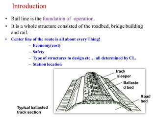
This document discusses various aspects of rail line design including track geometry, alignment, and cant. It defines key terms like plane section, longitudinal section, horizontal alignment, vertical alignment, and cant. It describes different types of tracks like straight tracks, circular curves, and transition curves. It explains how curve radius, superelevation (cant), cant transitions, and cant deficiency impact train speed and safety. Maximum speeds are determined based on factors like curve radius, cant, lateral acceleration limits, and vehicle specifications.

1. DEBRE MARKOS UNIVERSITY
INSTITUTE OF TECHNOLOGY
SCHOOL OF CIVIL AND WATER RESOURCE ENGINEERING
Chapter 2 Rail Line and Subgrade
Biniyam A 2022

2. Contents
• Economic survey and route selection of railway line
• Plane section design
• Longitudinal section design

3. Introduction
• Rail line is the foundation of operation.
• It is a whole structure consisted of the roadbed, bridge building
and rail.
• Center line of the route is all about everyThing!
– Economy(cost)
– Safety
– Type of structures to design etc… all determined by CL.
– Station location
track
sleeper
Ballaste
d bed
Road
bed
Typical ballasted
track section

4. Economic survey and route selection
Three stages：
Study and design
Feedback & evaluation
1. Earlier stage: research, survey and preliminary design work.
2. Basic construction stage ：first to do the measurement,
technical design and construction design, then begin to
construct it, finally check it into production.
3. Effect of feedback：several years later, to evaluate the
design and construction quality by investigate the engineering
quality, technical index and economic benefits.
Construction + maintenance

5. Route selection…
Route selection criteria：
- shortest , direct route,
- detour unsuitable geology, link important sites
- Cost effective (user & construction)
- Minimum earthwork,
- locally materials,
- Environmental friendly
- aesthetic value etc.
Balancing these
parameters and
requirements
target

6. Track geometry components
• An important aspect of construction is track geometry
• The projection of the track alignment on horizontal plane: Horizontal
alignment
• The projection of the track alignment on vertical plane: Vertical
alignment
Track geometry
Theoretical
(designed) track
Irregularity
(track quality)
• Gauge
• Horizontal alignment
• Cant
• Vertical alignment

7. Track alignment
The track alignment is explicitly or
implicitly defined in a coordinate
system
• The planar projection of center
line is called plane section of
the rail; and its vertical
projection is called
longitudinal section of the rail.
• The plane section of the rail is
consisted of straight line and
curve (circular curve and
easement curve).
• In the vertical direction:
gradients and vertical curves
and transition gradients
Vertical (Z)
North (X)
East (Y)
Longitudinal distance
Spacecurve
Projection

8. Locus of center of gravity position
of car body exists will take three
trajectories:
① curvature is zero: straight line；
② curvature is constant: circle curve；
③ curvature is variable: transition curve.
The main components of
Plane design:
1. Curves
2. Tangent/ straight lines
3. Easement/spiral curves
4. superelevation
1. Plane design
8

9. The curve is set when the line turns or
when two straight lines intersect.
curve radius (R),
corner curve (α),
curve length (L)
Tangent length (T),
easement curve length (Lo) .
Constituent parts of the curve
Types of curves
- simple/single
- common
Single curve
tangent length:
curve length:
External length:
9

10. 𝐿 =
𝜋 𝛼 − 2𝛽𝑜 𝑅
180
+ 2𝑙𝑜 ≈
𝜋𝛼𝑅
180
+ 𝑙𝑜 𝑚
𝐸 = 𝑅 + 𝑃 𝑠𝑒𝑐
𝛼
2
− 𝑅 𝑚
𝑇 = 𝑅 + 𝑃 𝑡𝑎𝑛
𝛼
2
+ 𝑚 𝑚
𝑚 =
𝑙𝑜
2
−
𝑙𝑜
3
240𝑅2
≈
𝑙𝑜
2 𝑚
𝑝 =
𝑙𝑜
2
24𝑅
(𝑚)
Common curve
10
When considering Easement curve:

11. Straight tracks (tangent tracks)
Straight tracks (sometimes “tangent tracks”)
• Horizontal curvature (change of direction
per unit length of the track) is zero
• Shortest length between two points
• No quasi-static lateral acceleration, no
need for cant
• Smallest possible gap between a train and
a platform
• Easy to check the train doors at a platform
• Possible to guide tamping machines with
laser beams
• Easy to install switches and crossings

12. Straight tracks
• There is no requirement for limiting
the length of straight track, only
minimum length
• The world’s longest straight track:
Australia, 478 km
• The longest straight track in Norway:
Kvineshei tunnel, 9020 m
(www.jernbaneverket.no)

13. Circular curve
Circular curves (sometimes “full curves”) with constant curve radius, R
• Constant horizontal curvature (change of direction per unit length of
the track)
• Constant quasi-static lateral acceleration (if the train runs at constant
speed)
Sign rules: Track standards use to have no sign rules. Software use
minus values for left hand curves (in the direction of the chainage).
Hence: -20000 meter is a larger radius than -200 meter

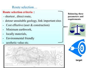
14. Circular curve
• The minimum radius is determined by the speed
– 30-60 m for tramways/metro lines
‐ 60-90 m on industrial railways
‐ Line speed for tramways/metro varies between 40 to 80 km/h
Recommended and minimum horizontal curve radius for v > 200 km/h:
Speed [km/h] 200 250 280 300 330 350
Recommended radius [m] 3200 5000 6300 7200 8700 9800
Minimum radius [m] 1888 2950 3700 4248 5140 5782
Note: use integer values for radius and not
larger than 99999 m

15. Circular curve
• There area also speed-independent criteria
– There is a minimum radius for tracks in platforms and turnouts
(Minimum radius for platform tracks R = 300
All vehicles must be able to run on R = 150 m (UIC)
– Minimum radius for no gauge widening R = 200 m
– Minimum radius for CWR R = 250 - 300 m
• Minimum length of curves and tangent tracks - Lmin > 0.4v
• Minimum radius for mainline tracks R ≥ 300 m

16. Circular curve
• The choice of the curve radius also depends on the characteristic of the
bogie
Tight curves and wide curve
Soft and rigid bogie suspension
Principal figure on how rails wear in curves

17. Circular curve effects
A vehicle running in a curve with radius R and speed v
experiences a centrifugal lateral acceleration a = v2/R this results
undesirable effects:
• possible passenger discomfort and noise nuisance
• possible displacement of wagon loads
• risk of vehicles overturning
• risk of derailment by wheel climbing or loosening of rail fastenings

18. Circular curve effects
Corrective measures for the curving phenomena:
• Increase the radius of curvature, R
• Use superelevation (cant) to compensate the lateral acceleration by
the gravity
• Reduction in train speed – not the best option

19. SUPERELEVATION (CANT)

20. Superelevation (cant)
• Cant is a corrective measure for the curving phenomena to compensate the
lateral acceleration
α

21. Applied cant (sometimes “superelevation”) is the amount of which one
running rail is raised above the other inner rail
• On curves, positive cant indicates that the outer rail is raised above
the inner rail
Superelevation (cant)

22. Equilibrium cant
m.v2
R
x
y
m.g
α
Fc
Fg
g = gravity = 9.81 (m/s/s)
R = curve radius (m)
α = cant angle (rad)
v = vehicle speed (m/s)
s = track width (1500 mm)
m = total mass of the vehicle
Fnet
h mv2
sv2
;
Therefore at balanced speed the cant
mv2
mgh
The equilibrium cant expressed in mm
net c g
mv2
F  F  F ;
Fc  cos; Fg  mg sin;
R
mgh
R
For small angle   ; F 
s c
; Fg 
s
gh
R s
v2
R s
At balanced speed Fnet  0 so
h 
gR
  
11.8v2
(km/h)
hth (mm) 
R(m)

23. Track plane acceleration
𝑣2
ℎ
𝑎𝑦 ≈
𝑅
− 𝑔 ∙
𝑠
• In case of quasistatic curving: track plane acceleration is 𝑎𝑦, and the
acceleration normal to the track plane is 𝑎𝑧
𝑣2
𝑎𝑦 =
𝑅
∙ 𝑐𝑜𝑠𝛼 − 𝑔 ∙ 𝑠𝑖𝑛𝛼
𝑣𝑒𝑞 =
• For a given cant an equilibrium
or balanced speed 𝑣𝑒𝑞, (𝑎𝑦 = 0)
𝑅𝑔ℎ
𝑠

24. Maximum speed in curves
• The important formula
𝑣2
− 𝑔 ∙ ℎ
= 𝑎 ≤ 𝑎
𝑅 𝑠 𝑦 𝑦,𝑚𝑎𝑥
 𝑣𝑚𝑎𝑥 =
𝑠
𝑔ℎ
+ 𝑎𝑦 ,𝑚𝑎
𝑥
∙ 𝑅
𝑎𝑦,𝑚𝑎𝑥 Maximum allowed uncompensated lateral acceleration

25. Applied cant limits
• Maximum applied cant on normal lines for high speed lines

26. Applied cant & cant deficiency
• For a number of trains the cant is
either too much or not enough
• Too much cant wear the inner wheel-
rail and increase friction on wheel
flange and increases the tractive
power required
• Too less cant causes large increase in
wear on the high rail
• Not enough cant creates transvers
force which is detrimental for both
safety and comfort (risk for
derailment and track displacement)

27. Cant deficiency (hd)
• Cant deficiency exists when the vehicle is travelling above balancing speed,
insufficient cant angle to cancel out lateral curving force
• The difference between the theoretical value of cant for maximum speed and the
applied value of cant
hd = ht (vmax) - ha < hd_all
𝑣2
𝑅
ℎ
𝑠
− 𝑔 ∙ 𝑎
= 𝑎𝑦
h +h
𝑣2
𝑅 𝑠
− 𝑔 ∙ 𝑎 d = 0
• The non compensated acceleration will be: ay = hd g/s
• With a non compensated acceleration of 1 m/s2 (maximum limit) and axle load
of 22.5 t, the quasi-static lateral load on the track is 22.5 kN

28. Cant deficiency and maximum speed
• The maximum non compensated acceleration ad,𝑚𝑎𝑥 expressed in terms of
maximum cant deficiency hd_max
ay,𝑚𝑎𝑥 = 𝑔 hd,max
𝑠
Gives the maximum speed in circular curve expressed with hd_max
𝑔
𝑠
ℎ + hd,𝑚𝑎𝑥
𝑣 = ∙ 𝑅
hd,𝑚𝑎𝑥 Maximum allowable cant deficiency

29. Example
• Given R=1600 m, s=1500 mm, h=150𝑚𝑚 g=10 m/s2, 𝑎𝑦,𝑚𝑎𝑥
=0.85 m/s2
• Balanced speed
𝑒
𝑞
𝑣 =
𝑅𝑔ℎ
𝑠
=
1500𝑚𝑚
1600𝑚∙10𝑚/𝑠2
∙150𝑚𝑚
= 40 m/s = 144 km/h
• maximum speed
𝑣2 ℎ
− 𝑔 ∙ = 𝑎𝑦,𝑚𝑎𝑥
𝑅 𝑠
𝑣𝑚𝑎𝑥 = 𝑠
𝑔ℎ
+ 𝑎𝑦 ,𝑚𝑎
𝑥
∙ 𝑅 =
1500
10∙150
+ 0.85 1600 = 54 m/s
= 195 km/h

30. Example
• Given v=240 km/h, s=1500 mm, h = 150 mm, g=10m/s2,
𝑎𝑦,𝑚𝑎𝑥=0.85 m/s2
𝑣2
− 𝑔 ∙ ℎ𝑚𝑎𝑥
= 𝑎
𝑅 𝑠 𝑦,𝑚𝑎𝑥
𝑣2
𝑅 = 𝑔ℎ𝑚𝑎𝑥
+ 𝑎𝑦,𝑚𝑎𝑥
240
3.6
2
= 10*150
𝑠 1500
+ 0.85
= 𝟐𝟒𝟎𝟎 𝐦
 High speed – large curve radius

31. Cant deficiency limits
• Limits for cant deficiency 𝑎𝑦,𝑚𝑎𝑥 𝑜𝑟 ℎ𝑑,𝑚𝑎𝑥 takes into account forces in
the wheel/rail interface as well as comfort or load displacements and safety
against derailment
• Avehicle must be tested and approved for its permissible cant deficiency,
according to procedures in UIC 518 or EN 14363
• Limits for train categories in Europe ranges from 92 mm (certain freight
cars) to 300 mm (tilting trains)

32. Santiago de Compostela, Spania, 24.
juli 2013

33. Santiago de Compostela, Spania, 24.
juli 2013
Geometry parameters and speed:
• Given: R = 300 m, h = 150 mm
• Recommended speed: V = 80 km/t  hd = 100 mm
• Real speed: V = 190 km/t  hd = 1271 mm ;
This corresponds to the lateral acceleration of ay ≈ 9,3 m/s2
The consequence 

34. Cant excess (he)
• Cant excess exists when the vehicle speed is lower than the balanced speed
• This can result in reduced passenger comfort but also a risk of roll-over for
vehicles with a high centre of gravity travelling at low speed, such as freight
vehicles
• The difference between the applied value of cant and the theoretical value
of cant for minimum speed
he = ha - hth (Vmin)
Cant excess he limits:
• Tracks with radius > 1000 m : Max. 100 mm
• Tracks with radius < 1000 m : Max. 70 mm

35. TRANSITION CURVES

36. • On a straight line, curvature is zero, while on a curve of radius R
curvature is 1/R
• Transition curves also introduce gauge widening
Often desired to have integer values for the lengths of transition curves
Transition curves

37. CANT TRANSITION

38. Cant transitions
Cant transitions (sometimes “superelevation ramps”):
• The transition between straight and curved sections requires variation of
cant
• The cant is changing as a function of chainage
• At tangent points, connected elements should have the same cant value
• Normally, the mathematical form for a cant transition is the same as for the
transition curve. Hence, for clothoids, the cant transitions are linear

39. Cant transitions
Cant transitions (sometimes “superelevation ramps”):
• Cant is introduced by means of transition gradients 𝜌 = ∆ℎ
∆𝐿
• In many railways the maximum cant is limited to 150-160 mm
• As to the alignment, the cant variation is one of the major causes for lateral
vibration in railway vehicle
In many countries, cant transitions on straight tracks and circular curves are
acceptable only in diverging tracks near a canted turnout

40. Cant transitions
• Cant transitions should normally coincide with transition curves (having
the same length and tangent points)
Criteria for cant transitions:
• Ageneral maximum limit of cant gradient ∆h/∆L < 1/400 (2.5%0) taking
into account wheel unloading ---- for h=150mm, min Lt = 60 m

41. Rate of change of cant ∆𝑫 will occur instead of an abrupt change of
applied cant, where transition curves are used
Rate of change of cant is defined as change in cant per time ∆𝐷 = ∆ℎ
∆𝑡
• Alimit for rate of change of cant (in mm/s),
dh/dt = ∆ha * V / (Lh * 3.6) ≤ (dha/dt)lim= ∆𝐷𝑚𝑎𝑥
Lh≥ ha* V / ∆𝑫𝒎𝒂𝒙
– Typical values for the limit is in the range 28-70 mm/s
Rate of change of cant

42. Rate of change of lateral acceleration
Rate of change of lateral acceleration (jerk) 𝛙:
Jerk is defined as change in non-compensated acceleration per time
𝜓 =
day
d𝑡
∆ay/∆t =ay*v/Lh ≤ (day/dt)lim= 𝜓𝑚𝑎𝑥
Lh≥ ay*v/𝜓𝑚𝑎𝑥

43. Transition curve and cant transition length
• There are three requiremnts
1. Requirment for maximum cant transition,
considering risk for derailment
1
𝐿 ≥
ℎ
𝜌𝑚𝑎
𝑥
2. Requiremnt for rate of change of cant
transition, considering comfort
2
𝐿 ≥ 𝑣 ∙
ℎ
∆𝐷𝑚𝑎
𝑥
3. Requiremnt to jerk, also considering
comfort
3
𝐿 ≥ 𝑣 ∙
ay
𝜓𝑚𝑎
𝑥

44. Example: Transition curve length
Given V= 180 km/h (50 m/s), h= 100 mm, 𝑎𝑦 = 𝑎𝑦,𝑚𝑎𝑥=0.65 m/s2
• Requirment 1
1
𝐿 ≥
ℎ
𝜌𝑚𝑎
𝑥
100
= = 40.0 m
2.5
• Requirment 2
2
𝐿 ≥ 𝑣 ∙
ℎ
∆𝐷𝑚𝑎
𝑥
100
= 50 ∙ = 178.6 m
28
• Requirment 3
3
𝐿 ≥ 𝑣 ∙
𝑎𝑦
𝜓𝑚𝑎
𝑥
0.65
= 50 ∙ = 203.1 m
0.16
The rquirment for jerk will govern the design L=203.1 m

45. Example: Transition curve length when 𝑎𝑦 is
not given
Given R = 1000 m, V= 90 km/h (25 m/s), h= 60 mm
• Requirment 1
1
𝐿 ≥
ℎ
𝜌𝑚𝑎
𝑥
60
= = 24.0 m
2.5
• Requirment 2
2
𝐿 ≥ 𝑣 ∙
ℎ
∆𝐷𝑚𝑎
𝑥
60
= 25 ∙ = 53.6 m
28
• Requirment 3 msut be calculated
𝑣2
𝑅
𝑎𝑦 = − 𝑔 ∙ =
ℎ 252
𝑠 1000
− 9.81 ∙
60
1500
= 0.233 m/s2 ≤ 𝑎𝑦,𝑚𝑎𝑥 − 𝑂𝐾!
3
𝐿 ≥ 𝑣 ∙
𝑎𝑦
𝜓𝑚𝑎
𝑥
0.233
= 25 ∙ = 36.3 m
0.16
L= 53.6 m