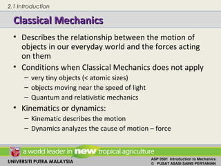
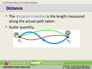
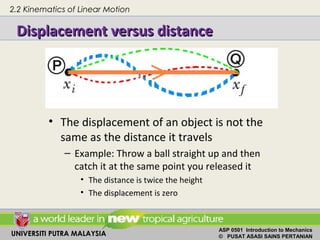
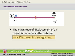
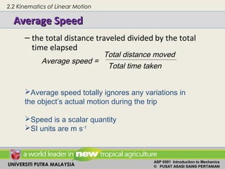
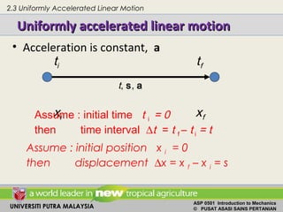
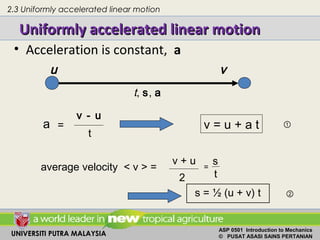
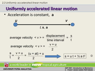
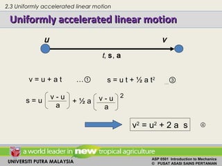
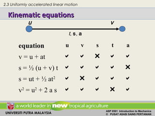
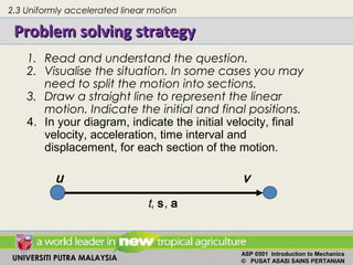
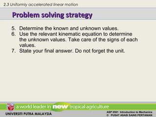
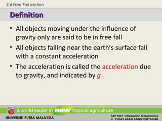
UNIVERSITI PUTRA MALAYSIA
ASP 0501 Introduction to Mechanics
© PUSAT ASASI SAINS PERTANIAN06/15/14UNIVERSITI PUTRA MALAYSIA
ASP 0501 Introduction to Mechanics
© PUSAT ASASI SAINS PERTANIAN
CHAPTER 2: Linear Kinematics
2.3
2.2
2.1
2.4
2.5
UNIVERSITI PUTRA MALAYSIA
ASP 0501 Introduction to Mechanics
© PUSAT ASASI SAINS PERTANIAN
KINEMATICS OF LINEAR MOTIONKINEMATICS OF LINEAR MOTION
• define and calculate displacement, velocity
and acceleration.
• use linear kinematic equations for uniform
acceleration
• solve free fall problems
• solve projectile motion problems
LEARNING OUTCOMES
After completing this chapter you must be able to:
UNIVERSITI PUTRA MALAYSIA
ASP 0501 Introduction to Mechanics
© PUSAT ASASI SAINS PERTANIAN
Classical MechanicsClassical Mechanics
• Describes the relationship between the motion of
objects in our everyday world and the forces acting
on them
• Conditions when Classical Mechanics does not apply
– very tiny objects (< atomic sizes)
– objects moving near the speed of light
– Quantum and relativistic mechanics
• Kinematics or dynamics:
– Kinematic describes the motion
– Dynamics analyzes the cause of motion – force
2.1 Introduction
UNIVERSITI PUTRA MALAYSIA
ASP 0501 Introduction to Mechanics
© PUSAT ASASI SAINS PERTANIAN
Sir Isaac NewtonSir Isaac Newton
• 1642 – 1727
• Formulated basic
concepts and laws of
mechanics
• Universal Gravitation
• Calculus
• Light and optics
2.1 Introduction
UNIVERSITI PUTRA MALAYSIA
ASP 0501 Introduction to Mechanics
© PUSAT ASASI SAINS PERTANIAN
KinematicsKinematics
• The branch of physics involving the motion of
an object and the relationship between that
motion and other physics concepts
• Kinematics is a part of dynamics
– description of motion
– Not concerned with the cause of the motion
2.1 Introduction
UNIVERSITI PUTRA MALAYSIA
ASP 0501 Introduction to Mechanics
© PUSAT ASASI SAINS PERTANIAN
Types of MotionTypes of Motion
• Translational motion: change of position
– Linear motion:
• One dimensional, the x- or y-axis
– Curvilinear:
• Two dimensional, x-y axis
• Parabolic path
– Circular motion
• Circular path
2.1 Introduction
UNIVERSITI PUTRA MALAYSIA
ASP 0501 Introduction to Mechanics
© PUSAT ASASI SAINS PERTANIAN
Types of MotionTypes of Motion
• Repeated Motions:
– Rotation: change of orientation
– Rolling: change of position and orientation
– Simple harmonic motion
– Damped harmonic motion
– Wave motion
2.1 Introduction
UNIVERSITI PUTRA MALAYSIA
ASP 0501 Introduction to Mechanics
© PUSAT ASASI SAINS PERTANIAN
Position vectorPosition vector
• Defined in terms of a frame of reference
– Defines a point relative to a reference point.
Reference point
Reference point
An object that moves, means there is change in
position.
2.2 Kinematics of Linear Motion
UNIVERSITI PUTRA MALAYSIA
ASP 0501 Introduction to Mechanics
© PUSAT ASASI SAINS PERTANIAN
DisplacementDisplacement
• The displacement is the quantity that
determines final position from the initial
position of a moving object.
• Defined as the change in position
• f stands for final and i stands for initial
– The SI units are meters (m)
∆ = −
ur ur ur
f ix x x
Initial position
Final position
2.2 Kinematics of Linear Motion
UNIVERSITI PUTRA MALAYSIA
ASP 0501 Introduction to Mechanics
© PUSAT ASASI SAINS PERTANIAN
DisplacementDisplacement
• In linear motion, we may represent
linear displacement as
∆ = −
ur ur ur
f ix x x
2.2 Kinematics of Linear Motion
Initial position Final position
xi xf
UNIVERSITI PUTRA MALAYSIA
ASP 0501 Introduction to Mechanics
© PUSAT ASASI SAINS PERTANIAN
DisplacementDisplacement
• It is a vector quantity.
• The magnitude of displacement is the shortest
distance between the final position from the
initial position.
• The direction of displacement is from the
initial position to the final position
2.2 Kinematics of Linear Motion
UNIVERSITI PUTRA MALAYSIA
ASP 0501 Introduction to Mechanics
© PUSAT ASASI SAINS PERTANIAN
DistanceDistance
• The distance travelled is the length measured
along the actual path taken.
• Scalar quantity.
2.2 Kinematics of Linear Motion
UNIVERSITI PUTRA MALAYSIA
ASP 0501 Introduction to Mechanics
© PUSAT ASASI SAINS PERTANIAN
• The displacement of an object is not the
same as the distance it travels
– Example: Throw a ball straight up and then
catch it at the same point you released it
• The distance is twice the height
• The displacement is zero
2.2 Kinematics of Linear Motion
Displacement versus distanceDisplacement versus distance
UNIVERSITI PUTRA MALAYSIA
ASP 0501 Introduction to Mechanics
© PUSAT ASASI SAINS PERTANIAN
• The magnitude of displacement of an
object is the same as the distance
only if it travels in a straight line.
2.2 Kinematics of Linear Motion
Displacement versus distanceDisplacement versus distance
UNIVERSITI PUTRA MALAYSIA
ASP 0501 Introduction to Mechanics
© PUSAT ASASI SAINS PERTANIAN
Average SpeedAverage Speed
– the total distance traveled divided by the total
time elapsed
Average speed =
Total distance moved
Total time taken
Average speed totally ignores any variations in
the object’s actual motion during the trip
Speed is a scalar quantity
SI units are m s-1
2.2 Kinematics of Linear Motion
UNIVERSITI PUTRA MALAYSIA
ASP 0501 Introduction to Mechanics
© PUSAT ASASI SAINS PERTANIAN
Average VelocityAverage Velocity
• Rate of change of position (rate of
displacement)
• Average velocity
– Ratio of displacement to time taken.
• A vector quantity.
f i
f i
x xx
v
t t t
−∆
< > = =
∆ −
v
v
2.2 Kinematics of Linear Motion
UNIVERSITI PUTRA MALAYSIA
ASP 0501 Introduction to Mechanics
© PUSAT ASASI SAINS PERTANIAN
Average VelocityAverage Velocity
• A vector quantity.
• Direction will be the same as the
direction of the displacement
• The SI units of velocity are m s-1
2.2 Kinematics of Linear Motion
Initial position
Final position
UNIVERSITI PUTRA MALAYSIA
ASP 0501 Introduction to Mechanics
© PUSAT ASASI SAINS PERTANIAN
Average speed vs. Average velocityAverage speed vs. Average velocity
• Consider two cars taking the same time interval but on
different paths.
• Cars on both paths have the same average velocity since
they had the same displacement in the same time interval
• The car on the blue path will have a greater average
speed since the distance it traveled is larger
2.2 Kinematics of Linear Motion
UNIVERSITI PUTRA MALAYSIA
ASP 0501 Introduction to Mechanics
© PUSAT ASASI SAINS PERTANIAN
Instantaneous VelocityInstantaneous Velocity
• The velocity of an object at particular instant.
• The limit of the average velocity as the time
interval becomes infinitesimally short, or as the
time interval approaches zero
• The instantaneous velocity indicates what is
happening at every point of time of the motion.
∆ →
∆
≡
∆
lim
0t
x
v
t
2.2 Kinematics of Linear Motion
UNIVERSITI PUTRA MALAYSIA
ASP 0501 Introduction to Mechanics
© PUSAT ASASI SAINS PERTANIAN
Instantaneous VelocityInstantaneous Velocity
• The instantaneous velocity varies from point to
point.
• In magnitude or direction or both.
2.2 Kinematics of Linear Motion
UNIVERSITI PUTRA MALAYSIA
ASP 0501 Introduction to Mechanics
© PUSAT ASASI SAINS PERTANIAN
Instantaneous VelocityInstantaneous Velocity
• The instantaneous velocity normally written as:
– velocity at point …
– velocity at time …..
• The magnitude of the instantaneous velocity is commonly
known as the speed at that particular position (time).
2.2 Kinematics of Linear Motion
UNIVERSITI PUTRA MALAYSIA
ASP 0501 Introduction to Mechanics
© PUSAT ASASI SAINS PERTANIAN
Uniform VelocityUniform Velocity
• Uniform velocity is constant velocity
• The instantaneous velocities are always the same
– All the instantaneous velocities will also equal the average
velocity
constant=
∆
∆
=
t
x
v


2.2 Kinematics of Linear Motion
UNIVERSITI PUTRA MALAYSIA
ASP 0501 Introduction to Mechanics
© PUSAT ASASI SAINS PERTANIAN
AccelerationAcceleration
• The average acceleration is defined as the rate
at which the velocity changes
• The instantaneous acceleration is the limit of
the average acceleration as Δt approaches
zero
av
t
∆
=
∆
v
a
r
r
dt
vd
a
r
r
=
2.2 Kinematics of Linear Motion
UNIVERSITI PUTRA MALAYSIA
ASP 0501 Introduction to Mechanics
© PUSAT ASASI SAINS PERTANIAN
AccelerationAcceleration
• Rate of change of velocity
• Changing velocity (non-uniform) means an
acceleration is present
• Acceleration is the rate of change of the
velocity
• Units are m s-²
−∆
= =
∆ −
f i
f i
v vv
a
t t t
2.2 Kinematics of Linear Motion
UNIVERSITI PUTRA MALAYSIA
ASP 0501 Introduction to Mechanics
© PUSAT ASASI SAINS PERTANIAN
Ways an Object Might AccelerateWays an Object Might Accelerate
• The magnitude of the velocity (the speed) can
change
• The direction of the velocity can change
– Even though the magnitude is constant
• Both the magnitude and the direction can
change
2.2 Kinematics of Linear Motion
UNIVERSITI PUTRA MALAYSIA
ASP 0501 Introduction to Mechanics
© PUSAT ASASI SAINS PERTANIAN
Average AccelerationAverage Acceleration
• Vector quantity
• When the sign of the velocity and the
acceleration are the same (either positive or
negative), then the speed is increasing
• When the sign of the velocity and the
acceleration are in the opposite directions,
the speed is decreasing
2.2 Kinematics of Linear Motion
UNIVERSITI PUTRA MALAYSIA
ASP 0501 Introduction to Mechanics
© PUSAT ASASI SAINS PERTANIAN
Instantaneous AccelerationInstantaneous Acceleration
• The instantaneous acceleration is the actual
acceleration at any particular time or position.
• When the instantaneous accelerations are
always the same, the acceleration will be
uniform
– The instantaneous accelerations will all be equal
to the average acceleration
2.2 Kinematics of Linear Motion
UNIVERSITI PUTRA MALAYSIA
ASP 0501 Introduction to Mechanics
© PUSAT ASASI SAINS PERTANIAN
Graphical representation of VelocityGraphical representation of Velocity
• Velocity can be determined from a position-
time graph
• Average velocity equals the slope of the line
joining the initial and final positions
• An object moving with a constant velocity will
have a graph that is a straight line
2.2 Kinematics of Linear Motion
UNIVERSITI PUTRA MALAYSIA
ASP 0501 Introduction to Mechanics
© PUSAT ASASI SAINS PERTANIAN
Uniform velocity graphUniform velocity graph
• The straight line indicates
constant velocity
• The slope of the line is the
value of the average
velocity
• A positive gradient means
a positive velocity
• A negative gradient means
a negative velocity
2.2 Kinematics of Linear Motion
UNIVERSITI PUTRA MALAYSIA
ASP 0501 Introduction to Mechanics
© PUSAT ASASI SAINS PERTANIAN
Non uniform velocityNon uniform velocity
• The graph is a curve.
• The average velocity is the
slope of the blue line
joining the starting and
end points.
• The instantaneous
velocity is the tangent at
each point.
2.2 Kinematics of Linear Motion
UNIVERSITI PUTRA MALAYSIA
ASP 0501 Introduction to Mechanics
© PUSAT ASASI SAINS PERTANIAN
Non-uniform VelocityNon-uniform Velocity
Positive direction,
Increasing magnitude
Positive direction,
decreasing magnitude
Negative direction,
deccreasing magnitude
negative direction,
Increasing magnitude
time time
time time
2.2 Kinematics of Linear Motion
UNIVERSITI PUTRA MALAYSIA
ASP 0501 Introduction to Mechanics
© PUSAT ASASI SAINS PERTANIAN
Graphical representation of AccelerationGraphical representation of Acceleration
• Average acceleration is the slope of the line
connecting the initial and final velocities on a
velocity-time graph
• Instantaneous acceleration is the slope of the
tangent to the curve of the velocity-time graph
2.2 Kinematics of Linear Motion
UNIVERSITI PUTRA MALAYSIA
ASP 0501 Introduction to Mechanics
© PUSAT ASASI SAINS PERTANIAN
Acceleration: velocity – time graphAcceleration: velocity – time graph
dt
dv
a =
2.2 Kinematics of Linear Motion
UNIVERSITI PUTRA MALAYSIA
ASP 0501 Introduction to Mechanics
© PUSAT ASASI SAINS PERTANIAN
Displacement, Velocity and AccelerationDisplacement, Velocity and Acceleration
x∆
x∆
t
x
v
∆
∆
=
t
v
a
∆
∆
=
Change of position
Change of position
Time interval
Change of velocity
Time interval
2.2 Kinematics of Linear Motion
UNIVERSITI PUTRA MALAYSIA
ASP 0501 Introduction to Mechanics
© PUSAT ASASI SAINS PERTANIAN
Problem solving strategyProblem solving strategy
1. Read and understand the question.
2. Visualise the situation. In some cases you may
need to split the motion into sections.
3. Draw the vector diagram to represent the motion.
It is advisable to draw a separate diagrams for the
displacement vectors and velocity vectors.
4. If you need to determine the resultant vector, use
the problem strategy for vector additions.
5. Extract the relevant data from the question.
6. Use the relevant equation to find the required
quantity.
7. Solve the equation to calculate your answer.
8. State your final answer. Do not forget the unit.
2.2 Kinematics of Linear Motion
UNIVERSITI PUTRA MALAYSIA
ASP 0501 Introduction to Mechanics
© PUSAT ASASI SAINS PERTANIAN
Uniformly accelerated linear motionUniformly accelerated linear motion
• Acceleration is constant, a
ti tf
xi xfAssume : initial time t i = 0
then time interval ∆t = t f – t i = t
Assume : initial position x i = 0
then displacement ∆x = x f – x i = s
t, s, a
2.3 Uniformly Accelerated Linear Motion
UNIVERSITI PUTRA MALAYSIA
ASP 0501 Introduction to Mechanics
© PUSAT ASASI SAINS PERTANIAN
Uniformly accelerated linear motionUniformly accelerated linear motion
• Acceleration is constant, a
t
u v
Assume: Initial velocity u
Final velocity v
acceleration a =
Change in velocity
Time interval
=
v - u
t
2.3 Uniformly accelerated linear motion
UNIVERSITI PUTRA MALAYSIA
ASP 0501 Introduction to Mechanics
© PUSAT ASASI SAINS PERTANIAN
Uniformly accelerated linear motionUniformly accelerated linear motion
• Acceleration is constant, a
u v
t, s, a
a =
v - u
t
v = u + a t
average velocity < v > =
v + u
2
①
=
s
t
s = ½ (u + v) t ②
2.3 Uniformly accelerated linear motion
UNIVERSITI PUTRA MALAYSIA
ASP 0501 Introduction to Mechanics
© PUSAT ASASI SAINS PERTANIAN
Uniformly accelerated linear motionUniformly accelerated linear motion
• Acceleration is constant, a
u v
t, s, a
average velocity < v > =
v + u
2
average velocity < v > =
displacement
time interval
=
s
t
s
t
=
v + u
2
=
(u + at) + u
2
s = u t + ½ a t2 ③
2.3 Uniformly accelerated linear motion
UNIVERSITI PUTRA MALAYSIA
ASP 0501 Introduction to Mechanics
© PUSAT ASASI SAINS PERTANIAN
v = u + a t …① s = u t + ½ a t2
…③
Uniformly accelerated linear motionUniformly accelerated linear motion
v - u
a
v - u
a
s = u + ½ a
2
v2
= u2
+ 2 a s
u v
t, s, a
④
2.3 Uniformly accelerated linear motion
UNIVERSITI PUTRA MALAYSIA
ASP 0501 Introduction to Mechanics
© PUSAT ASASI SAINS PERTANIAN
Kinematic equationsKinematic equations
equation u v s t a
v = u + at     
s = ½ (u + v) t     
s = ut + ½ at2     
v2
= u2
+ 2 a s     
u v
t, s, a
2.3 Uniformly accelerated linear motion
UNIVERSITI PUTRA MALAYSIA
ASP 0501 Introduction to Mechanics
© PUSAT ASASI SAINS PERTANIAN
Problem solving strategyProblem solving strategy
2.3 Uniformly accelerated linear motion
1. Read and understand the question.
2. Visualise the situation. In some cases you may
need to split the motion into sections.
3. Draw a straight line to represent the linear
motion. Indicate the initial and final positions.
4. In your diagram, indicate the initial velocity, final
velocity, acceleration, time interval and
displacement, for each section of the motion.
u v
t, s, a
UNIVERSITI PUTRA MALAYSIA
ASP 0501 Introduction to Mechanics
© PUSAT ASASI SAINS PERTANIAN
Problem solving strategyProblem solving strategy
2.3 Uniformly accelerated linear motion
5. Determine the known and unknown values.
6. Use the relevant kinematic equation to determine
the unknown values. Take care of the signs of each
values.
7. State your final answer. Do not forget the unit.
UNIVERSITI PUTRA MALAYSIA
ASP 0501 Introduction to Mechanics
© PUSAT ASASI SAINS PERTANIAN
DefinitionDefinition
• All objects moving under the influence of
gravity only are said to be in free fall
• All objects falling near the earth’s surface fall
with a constant acceleration
• The acceleration is called the acceleration due
to gravity, and indicated by g
2.4 Free Fall Motion
UNIVERSITI PUTRA MALAYSIA
ASP 0501 Introduction to Mechanics
© PUSAT ASASI SAINS PERTANIAN
Acceleration due to GravityAcceleration due to Gravity
• Symbolized by g
• g = 9.81 m s-2
(constant)
• g is always directed downward
– toward the center of the earth
• Ignoring air resistance and assuming g doesn’t
vary with altitude over short vertical
distances, free fall is constantly accelerated
motion
2.4 Free Fall Motion
UNIVERSITI PUTRA MALAYSIA
ASP 0501 Introduction to Mechanics
© PUSAT ASASI SAINS PERTANIAN
Kinematic equations for free fall motionKinematic equations for free fall motion
equation u v h t g
v = u + (-g) t     
h = ½ (u + v) t     
h = ut + ½ (-g) t2     
v2
= u2
+ 2 (-g) h     
u
v
- g
h
t
Reference direction: positive upwards
2.4 Free Fall Motion
UNIVERSITI PUTRA MALAYSIA
ASP 0501 Introduction to Mechanics
© PUSAT ASASI SAINS PERTANIAN
Object thrown vertically upwardObject thrown vertically upward
• Initial velocity is not zero
• Let up be positive
• Use the kinematic equations
v ( + ve)
a (- ve)
t ( +ve)
h ( +ve)
u ( + ve)
v = u + (− g ) t
h = u t + ½ (− g) t 2
v2
= u2
+ 2 (− g) h
g
2.4 Free Fall Motion
UNIVERSITI PUTRA MALAYSIA
ASP 0501 Introduction to Mechanics
© PUSAT ASASI SAINS PERTANIAN
Free Fall – an object droppedFree Fall – an object dropped
• Let up be positive
• Use the kinematic equations
u (-ve)
a = - g
t ( +ve)
h ( -ve)
V ( -ve)
(- v) = (- u) + (- g) t
(-h) = (- u) t + ½ (-g) t 2
(- v2
) = (-u)2
+ 2 (-g) (-h)
2.4 Free Fall Motion
UNIVERSITI PUTRA MALAYSIA
ASP 0501 Introduction to Mechanics
© PUSAT ASASI SAINS PERTANIAN
Object thrown vertically upwardObject thrown vertically upward
• Initial velocity is upward.
• a = g = 9.80 ms-2
is always
downward everywhere in
the motion
• The instantaneous velocity
at the maximum height is
zero
v = 0
2.4 Free Fall Motion
UNIVERSITI PUTRA MALAYSIA
ASP 0501 Introduction to Mechanics
© PUSAT ASASI SAINS PERTANIAN
Object thrown vertically
upward and caught at the
same position.
Symmetrical Free FallSymmetrical Free Fall
Initial velocity = final velocity
but in opposite direction
Time to reach highest position =
time to drop to initial position
u v
tup tdown
2.4 Free Fall Motion
UNIVERSITI PUTRA MALAYSIA
ASP 0501 Introduction to Mechanics
© PUSAT ASASI SAINS PERTANIAN
Non-symmetrical Free FallNon-symmetrical Free Fall
• Object thrown vertically
upward and falls to a
lower level.
– Upward and downward
portions
2.4 Free Fall Motion
UNIVERSITI PUTRA MALAYSIA
ASP 0501 Introduction to Mechanics
© PUSAT ASASI SAINS PERTANIAN
Problem solving strategyProblem solving strategy
2.4 Free Fall Motion
1. Read and understand the question.
2. Visualise the situation. In some cases you may need to
split the motion into upward and downward sections.
3. Draw a vertical straight line to represent the free fall
motion. Indicate the initial and final levels.
4. In your diagram, indicate the initial velocity, final
velocity, acceleration, time interval and displacement,
for each section of the motion.
5. Determine the known and unknown values.
6. Use the relevant kinematic equation to determine the
unknown values. Take care of the signs of each values.
7. State your final answer. Do not forget the unit.
UNIVERSITI PUTRA MALAYSIA
ASP 0501 Introduction to Mechanics
© PUSAT ASASI SAINS PERTANIAN
Projectile MotionProjectile Motion
• An object may move in both
the x and y directions
simultaneously
– It moves in two
dimensions
• The form of two dimensional
motion we will deal with is
called projectile motion
2.5 Projectile Motion
UNIVERSITI PUTRA MALAYSIA
ASP 0501 Introduction to Mechanics
© PUSAT ASASI SAINS PERTANIAN
Projectile Motion - accelerationProjectile Motion - acceleration
• y-direction
– free fall problem,
acceleration ay = g
(downward)
– Uniformly accelerated
linear motion, so the
motion equations all
hold
• x-direction
– Uniform motion
– ax= 0
2.5 Projectile Motion
UNIVERSITI PUTRA MALAYSIA
ASP 0501 Introduction to Mechanics
© PUSAT ASASI SAINS PERTANIAN
Projectile Motion – initial velocityProjectile Motion – initial velocity
• The initial velocity can be resolve into its x-
(horizontal) and y- (vertical) components
–
v
θ
V cos θ
V sin θ
2.5 Projectile Motion
UNIVERSITI PUTRA MALAYSIA
ASP 0501 Introduction to Mechanics
© PUSAT ASASI SAINS PERTANIAN
Projectile Motion – velocityProjectile Motion – velocity
• The velocity x- and y-directions of motion are completely independent of
each other
• The velocity can be resolve into its horizontal (x-) and vertical (y-)
components.
Velocity components
2.5 Projectile Motion
UNIVERSITI PUTRA MALAYSIA
ASP 0501 Introduction to Mechanics
© PUSAT ASASI SAINS PERTANIAN
Velocity of the ProjectileVelocity of the Projectile
• The velocity of the projectile at any point of its motion is the
vector sum of its x and y components at that point
2.5 Projectile Motion
UNIVERSITI PUTRA MALAYSIA
ASP 0501 Introduction to Mechanics
© PUSAT ASASI SAINS PERTANIAN
Velocity of the ProjectileVelocity of the Projectile
• The velocity of the projectile at any point of its
motion is the vector sum of its x and y
components at that point.
• The magnitude and direction of the velocity can
be calculated using:
2 2 1
tan y
x y
x
v
v v v and
v
θ −
= + =
2.5 Projectile Motion
UNIVERSITI PUTRA MALAYSIA
ASP 0501 Introduction to Mechanics
© PUSAT ASASI SAINS PERTANIAN
Projectile Motion – displacementProjectile Motion – displacement
► The displacement in x- and y-directions of motion are completely independent ofThe displacement in x- and y-directions of motion are completely independent of
each othereach other
► The displacement can be resolve into its horizontal (x-) and vertical (y-)
components.
Displacement components
2.5 Projectile Motion
UNIVERSITI PUTRA MALAYSIA
ASP 0501 Introduction to Mechanics
© PUSAT ASASI SAINS PERTANIAN
Projectile MotionProjectile Motion
Horizontal
component
Vertical
component
( + upward)
acceleration ax = 0 ay = - g
initial velocity vox = vo cos θ voy = vo sin θ
final velocity
(at max height)
vx = vox vy = 0
time interval t t
displacement x y horizontal
vo
θ
2.5 Projectile Motion
UNIVERSITI PUTRA MALAYSIA
ASP 0501 Introduction to Mechanics
© PUSAT ASASI SAINS PERTANIAN
Horizontal component Vertical component
( + upward)
acceleration ax = 0 ay = - g
initial velocity vox = vo cos θ voy = vo sin θ
final velocity
(at max height)
vx=vox vy = 0
time interval t t
displacement x y
Projectile MotionProjectile Motion
For vertical motion (+ upward):
② s = u t + ½ a t2
For horizontal motion:
② s = u t + ½ a t2
θ
θ
cos
)0(
2
1
)cos( 2
o
o
v
x
t
ttvx
=∴
+=
2
cos
)(
2
1
cos
)sin( 





−+





=
θθ
θ
oo
o
v
x
g
v
x
vy
θ
θ 22
2
cos2
tan
ov
gx
xy −= parabolic equation
y = ax2
+ bx + c
2.5 Projectile Motion
UNIVERSITI PUTRA MALAYSIA
ASP 0501 Introduction to Mechanics
© PUSAT ASASI SAINS PERTANIAN
Projectile MotionProjectile Motion
►The shape of the path is a parabolaThe shape of the path is a parabola
2.5 Projectile Motion
UNIVERSITI PUTRA MALAYSIA
ASP 0501 Introduction to Mechanics
© PUSAT ASASI SAINS PERTANIAN
Projectile MotionProjectile Motion
horizontal
vo
θ
At max height , vy = 0, using Eqn ①
v = u + at
0 = vo sin θ + (- g) T that is,
g
v
T o θsin
=
H
Horizontal
component
Vertical
component
( + upward)
acceleration ax = 0 ay = - g
initial velocity vox = vo cos θ voy = vo sin θ
final velocity
(at max height)
vx=vox vy = 0
time interval T
displacement H
2.5 Projectile Motion
UNIVERSITI PUTRA MALAYSIA
ASP 0501 Introduction to Mechanics
© PUSAT ASASI SAINS PERTANIAN
Projectile MotionProjectile Motion
At max height, using Eqn ②
s = u t + ½ (-g) t2
g
v
T o θsin
=
horizontal
vo
θ
g
v
g
v
g
g
v
vH
o
o
o
2
sin
sin
)(
2
1sin
sin
22
2
0
θ
θθ
θ
=






−+





=
Horizontal
component
Vertical component
( + upward)
acceleration ax = 0 ay = - g
initial velocity vox = vo cos θ voy = vo sin θ
final velocity
(at max height)
vx=vox vy = 0
time interval T
displacement H
H
2.5 Projectile Motion
UNIVERSITI PUTRA MALAYSIA
ASP 0501 Introduction to Mechanics
© PUSAT ASASI SAINS PERTANIAN
Projectile MotionProjectile Motion
Horizontal
component
Vertical component
( + upward)
acceleration ax = 0 ay = - g
initial velocity vox = vo cos θ voy = vo sin θ
final velocity
(at max height)
vx =vox = vo cos θ vy = 0
time interval 2 × T T
displacement R H
horizontal
vo
θ
At max horizontal displacement ,
using Eqn ② s = u t + ½ (-g) t2
g
v
T o θsin
=
g
v
g
v
g
v
g
v
vR
oo
oo
o
)2sin(sincos2
sin2
)0(
2
1sin2
cos
22
2
θθθ
θθ
θ
==






+





=
R
2.5 Projectile Motion
UNIVERSITI PUTRA MALAYSIA
ASP 0501 Introduction to Mechanics
© PUSAT ASASI SAINS PERTANIAN
Height and Range of the projectileHeight and Range of the projectile
• Maximum height: (y-axis)
• Range: (x-axis)
g
v
H o
2
sin22
θ
=
g
v
R o θ2sin
2
=
2.5 Projectile Motion
horizontal
vo
θ R
H
UNIVERSITI PUTRA MALAYSIA
ASP 0501 Introduction to Mechanics
© PUSAT ASASI SAINS PERTANIAN
Range and height of projectile motionRange and height of projectile motion
• Complementary
values of the initial
angle result in the
same range
– The heights will be
different
• The maximum range
occurs at a projection
angle of 45o
2.5 Projectile Motion
UNIVERSITI PUTRA MALAYSIA
ASP 0501 Introduction to Mechanics
© PUSAT ASASI SAINS PERTANIAN
Some Variations of Projectile MotionSome Variations of Projectile Motion
• An object may be fired
horizontally
• The initial velocity is all
in the x-direction
vo = vx and vy = 0
• All the general rules of
projectile motion apply
2.5 Projectile Motion
UNIVERSITI PUTRA MALAYSIA
ASP 0501 Introduction to Mechanics
© PUSAT ASASI SAINS PERTANIAN
Projectile MotionProjectile Motion
Horizontal component Vertical component
( + down)
acceleration ax = 0 ay = + g = 9.81 ms-2
initial velocity vox = 40.0 ms-1
voy = 0
final velocity vx = ? vy = ?
time interval T = ? T = ?
displacement R = ? H = 100 m
Find (a) the range R
(b) time to reach the ground
(c) velocity when touching the ground.
2.5 Projectile Motion
UNIVERSITI PUTRA MALAYSIA
ASP 0501 Introduction to Mechanics
© PUSAT ASASI SAINS PERTANIAN
Non-Symmetrical Projectile MotionNon-Symmetrical Projectile Motion
• Follow the general
rules for projectile
motion
• Break the y-direction
into parts
– up and down
– symmetrical back to
initial height and then
the rest of the height
2.5 Projectile Motion
UNIVERSITI PUTRA MALAYSIA
ASP 0501 Introduction to Mechanics
© PUSAT ASASI SAINS PERTANIAN
Non-Symmetrical Projectile MotionNon-Symmetrical Projectile Motion
Horizontal
component
Vertical component
( + up)
acceleration ax = 0 ay = − g = - 9.81
initial velocity vox = 20 cos 30 voy = 20 sin 30
final velocity vx = ? vy = 0
time interval t1 + t2 = ? t1 = ?
displacement X = ? h1 = ?
2.5 Projectile Motion
UNIVERSITI PUTRA MALAYSIA
ASP 0501 Introduction to Mechanics
© PUSAT ASASI SAINS PERTANIAN
Problem solving strategyProblem solving strategy
2.5 Projectile Motion
1. Read and understand the question.
2. Visualise the situation.
3. Draw the path of the projectile motion.
4. Resolved your vector quantities into vertical and
horizontal components
5. For each component, determine the known and
unknown values.
6. Use the relevant kinematic equation to determine the
unknown values.
Note: Horizontal component, a = 0
Vertical component, a = g = 9.81 ms-2
downward
7. State your final answer. Do not forget the unit.

Chap 2 linear kinematics

  • 1.
    UNIVERSITI PUTRA MALAYSIA ASP0501 Introduction to Mechanics © PUSAT ASASI SAINS PERTANIAN06/15/14UNIVERSITI PUTRA MALAYSIA ASP 0501 Introduction to Mechanics © PUSAT ASASI SAINS PERTANIAN CHAPTER 2: Linear Kinematics 2.3 2.2 2.1 2.4 2.5
  • 2.
    UNIVERSITI PUTRA MALAYSIA ASP0501 Introduction to Mechanics © PUSAT ASASI SAINS PERTANIAN KINEMATICS OF LINEAR MOTIONKINEMATICS OF LINEAR MOTION • define and calculate displacement, velocity and acceleration. • use linear kinematic equations for uniform acceleration • solve free fall problems • solve projectile motion problems LEARNING OUTCOMES After completing this chapter you must be able to:
  • 3.
    UNIVERSITI PUTRA MALAYSIA ASP0501 Introduction to Mechanics © PUSAT ASASI SAINS PERTANIAN Classical MechanicsClassical Mechanics • Describes the relationship between the motion of objects in our everyday world and the forces acting on them • Conditions when Classical Mechanics does not apply – very tiny objects (< atomic sizes) – objects moving near the speed of light – Quantum and relativistic mechanics • Kinematics or dynamics: – Kinematic describes the motion – Dynamics analyzes the cause of motion – force 2.1 Introduction
  • 4.
    UNIVERSITI PUTRA MALAYSIA ASP0501 Introduction to Mechanics © PUSAT ASASI SAINS PERTANIAN Sir Isaac NewtonSir Isaac Newton • 1642 – 1727 • Formulated basic concepts and laws of mechanics • Universal Gravitation • Calculus • Light and optics 2.1 Introduction
  • 5.
    UNIVERSITI PUTRA MALAYSIA ASP0501 Introduction to Mechanics © PUSAT ASASI SAINS PERTANIAN KinematicsKinematics • The branch of physics involving the motion of an object and the relationship between that motion and other physics concepts • Kinematics is a part of dynamics – description of motion – Not concerned with the cause of the motion 2.1 Introduction
  • 6.
    UNIVERSITI PUTRA MALAYSIA ASP0501 Introduction to Mechanics © PUSAT ASASI SAINS PERTANIAN Types of MotionTypes of Motion • Translational motion: change of position – Linear motion: • One dimensional, the x- or y-axis – Curvilinear: • Two dimensional, x-y axis • Parabolic path – Circular motion • Circular path 2.1 Introduction
  • 7.
    UNIVERSITI PUTRA MALAYSIA ASP0501 Introduction to Mechanics © PUSAT ASASI SAINS PERTANIAN Types of MotionTypes of Motion • Repeated Motions: – Rotation: change of orientation – Rolling: change of position and orientation – Simple harmonic motion – Damped harmonic motion – Wave motion 2.1 Introduction
  • 8.
    UNIVERSITI PUTRA MALAYSIA ASP0501 Introduction to Mechanics © PUSAT ASASI SAINS PERTANIAN Position vectorPosition vector • Defined in terms of a frame of reference – Defines a point relative to a reference point. Reference point Reference point An object that moves, means there is change in position. 2.2 Kinematics of Linear Motion
  • 9.
    UNIVERSITI PUTRA MALAYSIA ASP0501 Introduction to Mechanics © PUSAT ASASI SAINS PERTANIAN DisplacementDisplacement • The displacement is the quantity that determines final position from the initial position of a moving object. • Defined as the change in position • f stands for final and i stands for initial – The SI units are meters (m) ∆ = − ur ur ur f ix x x Initial position Final position 2.2 Kinematics of Linear Motion
  • 10.
    UNIVERSITI PUTRA MALAYSIA ASP0501 Introduction to Mechanics © PUSAT ASASI SAINS PERTANIAN DisplacementDisplacement • In linear motion, we may represent linear displacement as ∆ = − ur ur ur f ix x x 2.2 Kinematics of Linear Motion Initial position Final position xi xf
  • 11.
    UNIVERSITI PUTRA MALAYSIA ASP0501 Introduction to Mechanics © PUSAT ASASI SAINS PERTANIAN DisplacementDisplacement • It is a vector quantity. • The magnitude of displacement is the shortest distance between the final position from the initial position. • The direction of displacement is from the initial position to the final position 2.2 Kinematics of Linear Motion
  • 12.
    UNIVERSITI PUTRA MALAYSIA ASP0501 Introduction to Mechanics © PUSAT ASASI SAINS PERTANIAN DistanceDistance • The distance travelled is the length measured along the actual path taken. • Scalar quantity. 2.2 Kinematics of Linear Motion
  • 13.
    UNIVERSITI PUTRA MALAYSIA ASP0501 Introduction to Mechanics © PUSAT ASASI SAINS PERTANIAN • The displacement of an object is not the same as the distance it travels – Example: Throw a ball straight up and then catch it at the same point you released it • The distance is twice the height • The displacement is zero 2.2 Kinematics of Linear Motion Displacement versus distanceDisplacement versus distance
  • 14.
    UNIVERSITI PUTRA MALAYSIA ASP0501 Introduction to Mechanics © PUSAT ASASI SAINS PERTANIAN • The magnitude of displacement of an object is the same as the distance only if it travels in a straight line. 2.2 Kinematics of Linear Motion Displacement versus distanceDisplacement versus distance
  • 15.
    UNIVERSITI PUTRA MALAYSIA ASP0501 Introduction to Mechanics © PUSAT ASASI SAINS PERTANIAN Average SpeedAverage Speed – the total distance traveled divided by the total time elapsed Average speed = Total distance moved Total time taken Average speed totally ignores any variations in the object’s actual motion during the trip Speed is a scalar quantity SI units are m s-1 2.2 Kinematics of Linear Motion
  • 16.
    UNIVERSITI PUTRA MALAYSIA ASP0501 Introduction to Mechanics © PUSAT ASASI SAINS PERTANIAN Average VelocityAverage Velocity • Rate of change of position (rate of displacement) • Average velocity – Ratio of displacement to time taken. • A vector quantity. f i f i x xx v t t t −∆ < > = = ∆ − v v 2.2 Kinematics of Linear Motion
  • 17.
    UNIVERSITI PUTRA MALAYSIA ASP0501 Introduction to Mechanics © PUSAT ASASI SAINS PERTANIAN Average VelocityAverage Velocity • A vector quantity. • Direction will be the same as the direction of the displacement • The SI units of velocity are m s-1 2.2 Kinematics of Linear Motion Initial position Final position
  • 18.
    UNIVERSITI PUTRA MALAYSIA ASP0501 Introduction to Mechanics © PUSAT ASASI SAINS PERTANIAN Average speed vs. Average velocityAverage speed vs. Average velocity • Consider two cars taking the same time interval but on different paths. • Cars on both paths have the same average velocity since they had the same displacement in the same time interval • The car on the blue path will have a greater average speed since the distance it traveled is larger 2.2 Kinematics of Linear Motion
  • 19.
    UNIVERSITI PUTRA MALAYSIA ASP0501 Introduction to Mechanics © PUSAT ASASI SAINS PERTANIAN Instantaneous VelocityInstantaneous Velocity • The velocity of an object at particular instant. • The limit of the average velocity as the time interval becomes infinitesimally short, or as the time interval approaches zero • The instantaneous velocity indicates what is happening at every point of time of the motion. ∆ → ∆ ≡ ∆ lim 0t x v t 2.2 Kinematics of Linear Motion
  • 20.
    UNIVERSITI PUTRA MALAYSIA ASP0501 Introduction to Mechanics © PUSAT ASASI SAINS PERTANIAN Instantaneous VelocityInstantaneous Velocity • The instantaneous velocity varies from point to point. • In magnitude or direction or both. 2.2 Kinematics of Linear Motion
  • 21.
    UNIVERSITI PUTRA MALAYSIA ASP0501 Introduction to Mechanics © PUSAT ASASI SAINS PERTANIAN Instantaneous VelocityInstantaneous Velocity • The instantaneous velocity normally written as: – velocity at point … – velocity at time ….. • The magnitude of the instantaneous velocity is commonly known as the speed at that particular position (time). 2.2 Kinematics of Linear Motion
  • 22.
    UNIVERSITI PUTRA MALAYSIA ASP0501 Introduction to Mechanics © PUSAT ASASI SAINS PERTANIAN Uniform VelocityUniform Velocity • Uniform velocity is constant velocity • The instantaneous velocities are always the same – All the instantaneous velocities will also equal the average velocity constant= ∆ ∆ = t x v   2.2 Kinematics of Linear Motion
  • 23.
    UNIVERSITI PUTRA MALAYSIA ASP0501 Introduction to Mechanics © PUSAT ASASI SAINS PERTANIAN AccelerationAcceleration • The average acceleration is defined as the rate at which the velocity changes • The instantaneous acceleration is the limit of the average acceleration as Δt approaches zero av t ∆ = ∆ v a r r dt vd a r r = 2.2 Kinematics of Linear Motion
  • 24.
    UNIVERSITI PUTRA MALAYSIA ASP0501 Introduction to Mechanics © PUSAT ASASI SAINS PERTANIAN AccelerationAcceleration • Rate of change of velocity • Changing velocity (non-uniform) means an acceleration is present • Acceleration is the rate of change of the velocity • Units are m s-² −∆ = = ∆ − f i f i v vv a t t t 2.2 Kinematics of Linear Motion
  • 25.
    UNIVERSITI PUTRA MALAYSIA ASP0501 Introduction to Mechanics © PUSAT ASASI SAINS PERTANIAN Ways an Object Might AccelerateWays an Object Might Accelerate • The magnitude of the velocity (the speed) can change • The direction of the velocity can change – Even though the magnitude is constant • Both the magnitude and the direction can change 2.2 Kinematics of Linear Motion
  • 26.
    UNIVERSITI PUTRA MALAYSIA ASP0501 Introduction to Mechanics © PUSAT ASASI SAINS PERTANIAN Average AccelerationAverage Acceleration • Vector quantity • When the sign of the velocity and the acceleration are the same (either positive or negative), then the speed is increasing • When the sign of the velocity and the acceleration are in the opposite directions, the speed is decreasing 2.2 Kinematics of Linear Motion
  • 27.
    UNIVERSITI PUTRA MALAYSIA ASP0501 Introduction to Mechanics © PUSAT ASASI SAINS PERTANIAN Instantaneous AccelerationInstantaneous Acceleration • The instantaneous acceleration is the actual acceleration at any particular time or position. • When the instantaneous accelerations are always the same, the acceleration will be uniform – The instantaneous accelerations will all be equal to the average acceleration 2.2 Kinematics of Linear Motion
  • 28.
    UNIVERSITI PUTRA MALAYSIA ASP0501 Introduction to Mechanics © PUSAT ASASI SAINS PERTANIAN Graphical representation of VelocityGraphical representation of Velocity • Velocity can be determined from a position- time graph • Average velocity equals the slope of the line joining the initial and final positions • An object moving with a constant velocity will have a graph that is a straight line 2.2 Kinematics of Linear Motion
  • 29.
    UNIVERSITI PUTRA MALAYSIA ASP0501 Introduction to Mechanics © PUSAT ASASI SAINS PERTANIAN Uniform velocity graphUniform velocity graph • The straight line indicates constant velocity • The slope of the line is the value of the average velocity • A positive gradient means a positive velocity • A negative gradient means a negative velocity 2.2 Kinematics of Linear Motion
  • 30.
    UNIVERSITI PUTRA MALAYSIA ASP0501 Introduction to Mechanics © PUSAT ASASI SAINS PERTANIAN Non uniform velocityNon uniform velocity • The graph is a curve. • The average velocity is the slope of the blue line joining the starting and end points. • The instantaneous velocity is the tangent at each point. 2.2 Kinematics of Linear Motion
  • 31.
    UNIVERSITI PUTRA MALAYSIA ASP0501 Introduction to Mechanics © PUSAT ASASI SAINS PERTANIAN Non-uniform VelocityNon-uniform Velocity Positive direction, Increasing magnitude Positive direction, decreasing magnitude Negative direction, deccreasing magnitude negative direction, Increasing magnitude time time time time 2.2 Kinematics of Linear Motion
  • 32.
    UNIVERSITI PUTRA MALAYSIA ASP0501 Introduction to Mechanics © PUSAT ASASI SAINS PERTANIAN Graphical representation of AccelerationGraphical representation of Acceleration • Average acceleration is the slope of the line connecting the initial and final velocities on a velocity-time graph • Instantaneous acceleration is the slope of the tangent to the curve of the velocity-time graph 2.2 Kinematics of Linear Motion
  • 33.
    UNIVERSITI PUTRA MALAYSIA ASP0501 Introduction to Mechanics © PUSAT ASASI SAINS PERTANIAN Acceleration: velocity – time graphAcceleration: velocity – time graph dt dv a = 2.2 Kinematics of Linear Motion
  • 34.
    UNIVERSITI PUTRA MALAYSIA ASP0501 Introduction to Mechanics © PUSAT ASASI SAINS PERTANIAN Displacement, Velocity and AccelerationDisplacement, Velocity and Acceleration x∆ x∆ t x v ∆ ∆ = t v a ∆ ∆ = Change of position Change of position Time interval Change of velocity Time interval 2.2 Kinematics of Linear Motion
  • 35.
    UNIVERSITI PUTRA MALAYSIA ASP0501 Introduction to Mechanics © PUSAT ASASI SAINS PERTANIAN Problem solving strategyProblem solving strategy 1. Read and understand the question. 2. Visualise the situation. In some cases you may need to split the motion into sections. 3. Draw the vector diagram to represent the motion. It is advisable to draw a separate diagrams for the displacement vectors and velocity vectors. 4. If you need to determine the resultant vector, use the problem strategy for vector additions. 5. Extract the relevant data from the question. 6. Use the relevant equation to find the required quantity. 7. Solve the equation to calculate your answer. 8. State your final answer. Do not forget the unit. 2.2 Kinematics of Linear Motion
  • 36.
    UNIVERSITI PUTRA MALAYSIA ASP0501 Introduction to Mechanics © PUSAT ASASI SAINS PERTANIAN Uniformly accelerated linear motionUniformly accelerated linear motion • Acceleration is constant, a ti tf xi xfAssume : initial time t i = 0 then time interval ∆t = t f – t i = t Assume : initial position x i = 0 then displacement ∆x = x f – x i = s t, s, a 2.3 Uniformly Accelerated Linear Motion
  • 37.
    UNIVERSITI PUTRA MALAYSIA ASP0501 Introduction to Mechanics © PUSAT ASASI SAINS PERTANIAN Uniformly accelerated linear motionUniformly accelerated linear motion • Acceleration is constant, a t u v Assume: Initial velocity u Final velocity v acceleration a = Change in velocity Time interval = v - u t 2.3 Uniformly accelerated linear motion
  • 38.
    UNIVERSITI PUTRA MALAYSIA ASP0501 Introduction to Mechanics © PUSAT ASASI SAINS PERTANIAN Uniformly accelerated linear motionUniformly accelerated linear motion • Acceleration is constant, a u v t, s, a a = v - u t v = u + a t average velocity < v > = v + u 2 ① = s t s = ½ (u + v) t ② 2.3 Uniformly accelerated linear motion
  • 39.
    UNIVERSITI PUTRA MALAYSIA ASP0501 Introduction to Mechanics © PUSAT ASASI SAINS PERTANIAN Uniformly accelerated linear motionUniformly accelerated linear motion • Acceleration is constant, a u v t, s, a average velocity < v > = v + u 2 average velocity < v > = displacement time interval = s t s t = v + u 2 = (u + at) + u 2 s = u t + ½ a t2 ③ 2.3 Uniformly accelerated linear motion
  • 40.
    UNIVERSITI PUTRA MALAYSIA ASP0501 Introduction to Mechanics © PUSAT ASASI SAINS PERTANIAN v = u + a t …① s = u t + ½ a t2 …③ Uniformly accelerated linear motionUniformly accelerated linear motion v - u a v - u a s = u + ½ a 2 v2 = u2 + 2 a s u v t, s, a ④ 2.3 Uniformly accelerated linear motion
  • 41.
    UNIVERSITI PUTRA MALAYSIA ASP0501 Introduction to Mechanics © PUSAT ASASI SAINS PERTANIAN Kinematic equationsKinematic equations equation u v s t a v = u + at      s = ½ (u + v) t      s = ut + ½ at2      v2 = u2 + 2 a s      u v t, s, a 2.3 Uniformly accelerated linear motion
  • 42.
    UNIVERSITI PUTRA MALAYSIA ASP0501 Introduction to Mechanics © PUSAT ASASI SAINS PERTANIAN Problem solving strategyProblem solving strategy 2.3 Uniformly accelerated linear motion 1. Read and understand the question. 2. Visualise the situation. In some cases you may need to split the motion into sections. 3. Draw a straight line to represent the linear motion. Indicate the initial and final positions. 4. In your diagram, indicate the initial velocity, final velocity, acceleration, time interval and displacement, for each section of the motion. u v t, s, a
  • 43.
    UNIVERSITI PUTRA MALAYSIA ASP0501 Introduction to Mechanics © PUSAT ASASI SAINS PERTANIAN Problem solving strategyProblem solving strategy 2.3 Uniformly accelerated linear motion 5. Determine the known and unknown values. 6. Use the relevant kinematic equation to determine the unknown values. Take care of the signs of each values. 7. State your final answer. Do not forget the unit.
  • 44.
    UNIVERSITI PUTRA MALAYSIA ASP0501 Introduction to Mechanics © PUSAT ASASI SAINS PERTANIAN DefinitionDefinition • All objects moving under the influence of gravity only are said to be in free fall • All objects falling near the earth’s surface fall with a constant acceleration • The acceleration is called the acceleration due to gravity, and indicated by g 2.4 Free Fall Motion
  • 45.
    UNIVERSITI PUTRA MALAYSIA ASP0501 Introduction to Mechanics © PUSAT ASASI SAINS PERTANIAN Acceleration due to GravityAcceleration due to Gravity • Symbolized by g • g = 9.81 m s-2 (constant) • g is always directed downward – toward the center of the earth • Ignoring air resistance and assuming g doesn’t vary with altitude over short vertical distances, free fall is constantly accelerated motion 2.4 Free Fall Motion
  • 46.
    UNIVERSITI PUTRA MALAYSIA ASP0501 Introduction to Mechanics © PUSAT ASASI SAINS PERTANIAN Kinematic equations for free fall motionKinematic equations for free fall motion equation u v h t g v = u + (-g) t      h = ½ (u + v) t      h = ut + ½ (-g) t2      v2 = u2 + 2 (-g) h      u v - g h t Reference direction: positive upwards 2.4 Free Fall Motion
  • 47.
    UNIVERSITI PUTRA MALAYSIA ASP0501 Introduction to Mechanics © PUSAT ASASI SAINS PERTANIAN Object thrown vertically upwardObject thrown vertically upward • Initial velocity is not zero • Let up be positive • Use the kinematic equations v ( + ve) a (- ve) t ( +ve) h ( +ve) u ( + ve) v = u + (− g ) t h = u t + ½ (− g) t 2 v2 = u2 + 2 (− g) h g 2.4 Free Fall Motion
  • 48.
    UNIVERSITI PUTRA MALAYSIA ASP0501 Introduction to Mechanics © PUSAT ASASI SAINS PERTANIAN Free Fall – an object droppedFree Fall – an object dropped • Let up be positive • Use the kinematic equations u (-ve) a = - g t ( +ve) h ( -ve) V ( -ve) (- v) = (- u) + (- g) t (-h) = (- u) t + ½ (-g) t 2 (- v2 ) = (-u)2 + 2 (-g) (-h) 2.4 Free Fall Motion
  • 49.
    UNIVERSITI PUTRA MALAYSIA ASP0501 Introduction to Mechanics © PUSAT ASASI SAINS PERTANIAN Object thrown vertically upwardObject thrown vertically upward • Initial velocity is upward. • a = g = 9.80 ms-2 is always downward everywhere in the motion • The instantaneous velocity at the maximum height is zero v = 0 2.4 Free Fall Motion
  • 50.
    UNIVERSITI PUTRA MALAYSIA ASP0501 Introduction to Mechanics © PUSAT ASASI SAINS PERTANIAN Object thrown vertically upward and caught at the same position. Symmetrical Free FallSymmetrical Free Fall Initial velocity = final velocity but in opposite direction Time to reach highest position = time to drop to initial position u v tup tdown 2.4 Free Fall Motion
  • 51.
    UNIVERSITI PUTRA MALAYSIA ASP0501 Introduction to Mechanics © PUSAT ASASI SAINS PERTANIAN Non-symmetrical Free FallNon-symmetrical Free Fall • Object thrown vertically upward and falls to a lower level. – Upward and downward portions 2.4 Free Fall Motion
  • 52.
    UNIVERSITI PUTRA MALAYSIA ASP0501 Introduction to Mechanics © PUSAT ASASI SAINS PERTANIAN Problem solving strategyProblem solving strategy 2.4 Free Fall Motion 1. Read and understand the question. 2. Visualise the situation. In some cases you may need to split the motion into upward and downward sections. 3. Draw a vertical straight line to represent the free fall motion. Indicate the initial and final levels. 4. In your diagram, indicate the initial velocity, final velocity, acceleration, time interval and displacement, for each section of the motion. 5. Determine the known and unknown values. 6. Use the relevant kinematic equation to determine the unknown values. Take care of the signs of each values. 7. State your final answer. Do not forget the unit.
  • 53.
    UNIVERSITI PUTRA MALAYSIA ASP0501 Introduction to Mechanics © PUSAT ASASI SAINS PERTANIAN Projectile MotionProjectile Motion • An object may move in both the x and y directions simultaneously – It moves in two dimensions • The form of two dimensional motion we will deal with is called projectile motion 2.5 Projectile Motion
  • 54.
    UNIVERSITI PUTRA MALAYSIA ASP0501 Introduction to Mechanics © PUSAT ASASI SAINS PERTANIAN Projectile Motion - accelerationProjectile Motion - acceleration • y-direction – free fall problem, acceleration ay = g (downward) – Uniformly accelerated linear motion, so the motion equations all hold • x-direction – Uniform motion – ax= 0 2.5 Projectile Motion
  • 55.
    UNIVERSITI PUTRA MALAYSIA ASP0501 Introduction to Mechanics © PUSAT ASASI SAINS PERTANIAN Projectile Motion – initial velocityProjectile Motion – initial velocity • The initial velocity can be resolve into its x- (horizontal) and y- (vertical) components – v θ V cos θ V sin θ 2.5 Projectile Motion
  • 56.
    UNIVERSITI PUTRA MALAYSIA ASP0501 Introduction to Mechanics © PUSAT ASASI SAINS PERTANIAN Projectile Motion – velocityProjectile Motion – velocity • The velocity x- and y-directions of motion are completely independent of each other • The velocity can be resolve into its horizontal (x-) and vertical (y-) components. Velocity components 2.5 Projectile Motion
  • 57.
    UNIVERSITI PUTRA MALAYSIA ASP0501 Introduction to Mechanics © PUSAT ASASI SAINS PERTANIAN Velocity of the ProjectileVelocity of the Projectile • The velocity of the projectile at any point of its motion is the vector sum of its x and y components at that point 2.5 Projectile Motion
  • 58.
    UNIVERSITI PUTRA MALAYSIA ASP0501 Introduction to Mechanics © PUSAT ASASI SAINS PERTANIAN Velocity of the ProjectileVelocity of the Projectile • The velocity of the projectile at any point of its motion is the vector sum of its x and y components at that point. • The magnitude and direction of the velocity can be calculated using: 2 2 1 tan y x y x v v v v and v θ − = + = 2.5 Projectile Motion
  • 59.
    UNIVERSITI PUTRA MALAYSIA ASP0501 Introduction to Mechanics © PUSAT ASASI SAINS PERTANIAN Projectile Motion – displacementProjectile Motion – displacement ► The displacement in x- and y-directions of motion are completely independent ofThe displacement in x- and y-directions of motion are completely independent of each othereach other ► The displacement can be resolve into its horizontal (x-) and vertical (y-) components. Displacement components 2.5 Projectile Motion
  • 60.
    UNIVERSITI PUTRA MALAYSIA ASP0501 Introduction to Mechanics © PUSAT ASASI SAINS PERTANIAN Projectile MotionProjectile Motion Horizontal component Vertical component ( + upward) acceleration ax = 0 ay = - g initial velocity vox = vo cos θ voy = vo sin θ final velocity (at max height) vx = vox vy = 0 time interval t t displacement x y horizontal vo θ 2.5 Projectile Motion
  • 61.
    UNIVERSITI PUTRA MALAYSIA ASP0501 Introduction to Mechanics © PUSAT ASASI SAINS PERTANIAN Horizontal component Vertical component ( + upward) acceleration ax = 0 ay = - g initial velocity vox = vo cos θ voy = vo sin θ final velocity (at max height) vx=vox vy = 0 time interval t t displacement x y Projectile MotionProjectile Motion For vertical motion (+ upward): ② s = u t + ½ a t2 For horizontal motion: ② s = u t + ½ a t2 θ θ cos )0( 2 1 )cos( 2 o o v x t ttvx =∴ += 2 cos )( 2 1 cos )sin(       −+      = θθ θ oo o v x g v x vy θ θ 22 2 cos2 tan ov gx xy −= parabolic equation y = ax2 + bx + c 2.5 Projectile Motion
  • 62.
    UNIVERSITI PUTRA MALAYSIA ASP0501 Introduction to Mechanics © PUSAT ASASI SAINS PERTANIAN Projectile MotionProjectile Motion ►The shape of the path is a parabolaThe shape of the path is a parabola 2.5 Projectile Motion
  • 63.
    UNIVERSITI PUTRA MALAYSIA ASP0501 Introduction to Mechanics © PUSAT ASASI SAINS PERTANIAN Projectile MotionProjectile Motion horizontal vo θ At max height , vy = 0, using Eqn ① v = u + at 0 = vo sin θ + (- g) T that is, g v T o θsin = H Horizontal component Vertical component ( + upward) acceleration ax = 0 ay = - g initial velocity vox = vo cos θ voy = vo sin θ final velocity (at max height) vx=vox vy = 0 time interval T displacement H 2.5 Projectile Motion
  • 64.
    UNIVERSITI PUTRA MALAYSIA ASP0501 Introduction to Mechanics © PUSAT ASASI SAINS PERTANIAN Projectile MotionProjectile Motion At max height, using Eqn ② s = u t + ½ (-g) t2 g v T o θsin = horizontal vo θ g v g v g g v vH o o o 2 sin sin )( 2 1sin sin 22 2 0 θ θθ θ =       −+      = Horizontal component Vertical component ( + upward) acceleration ax = 0 ay = - g initial velocity vox = vo cos θ voy = vo sin θ final velocity (at max height) vx=vox vy = 0 time interval T displacement H H 2.5 Projectile Motion
  • 65.
    UNIVERSITI PUTRA MALAYSIA ASP0501 Introduction to Mechanics © PUSAT ASASI SAINS PERTANIAN Projectile MotionProjectile Motion Horizontal component Vertical component ( + upward) acceleration ax = 0 ay = - g initial velocity vox = vo cos θ voy = vo sin θ final velocity (at max height) vx =vox = vo cos θ vy = 0 time interval 2 × T T displacement R H horizontal vo θ At max horizontal displacement , using Eqn ② s = u t + ½ (-g) t2 g v T o θsin = g v g v g v g v vR oo oo o )2sin(sincos2 sin2 )0( 2 1sin2 cos 22 2 θθθ θθ θ ==       +      = R 2.5 Projectile Motion
  • 66.
    UNIVERSITI PUTRA MALAYSIA ASP0501 Introduction to Mechanics © PUSAT ASASI SAINS PERTANIAN Height and Range of the projectileHeight and Range of the projectile • Maximum height: (y-axis) • Range: (x-axis) g v H o 2 sin22 θ = g v R o θ2sin 2 = 2.5 Projectile Motion horizontal vo θ R H
  • 67.
    UNIVERSITI PUTRA MALAYSIA ASP0501 Introduction to Mechanics © PUSAT ASASI SAINS PERTANIAN Range and height of projectile motionRange and height of projectile motion • Complementary values of the initial angle result in the same range – The heights will be different • The maximum range occurs at a projection angle of 45o 2.5 Projectile Motion
  • 68.
    UNIVERSITI PUTRA MALAYSIA ASP0501 Introduction to Mechanics © PUSAT ASASI SAINS PERTANIAN Some Variations of Projectile MotionSome Variations of Projectile Motion • An object may be fired horizontally • The initial velocity is all in the x-direction vo = vx and vy = 0 • All the general rules of projectile motion apply 2.5 Projectile Motion
  • 69.
    UNIVERSITI PUTRA MALAYSIA ASP0501 Introduction to Mechanics © PUSAT ASASI SAINS PERTANIAN Projectile MotionProjectile Motion Horizontal component Vertical component ( + down) acceleration ax = 0 ay = + g = 9.81 ms-2 initial velocity vox = 40.0 ms-1 voy = 0 final velocity vx = ? vy = ? time interval T = ? T = ? displacement R = ? H = 100 m Find (a) the range R (b) time to reach the ground (c) velocity when touching the ground. 2.5 Projectile Motion
  • 70.
    UNIVERSITI PUTRA MALAYSIA ASP0501 Introduction to Mechanics © PUSAT ASASI SAINS PERTANIAN Non-Symmetrical Projectile MotionNon-Symmetrical Projectile Motion • Follow the general rules for projectile motion • Break the y-direction into parts – up and down – symmetrical back to initial height and then the rest of the height 2.5 Projectile Motion
  • 71.
    UNIVERSITI PUTRA MALAYSIA ASP0501 Introduction to Mechanics © PUSAT ASASI SAINS PERTANIAN Non-Symmetrical Projectile MotionNon-Symmetrical Projectile Motion Horizontal component Vertical component ( + up) acceleration ax = 0 ay = − g = - 9.81 initial velocity vox = 20 cos 30 voy = 20 sin 30 final velocity vx = ? vy = 0 time interval t1 + t2 = ? t1 = ? displacement X = ? h1 = ? 2.5 Projectile Motion
  • 72.
    UNIVERSITI PUTRA MALAYSIA ASP0501 Introduction to Mechanics © PUSAT ASASI SAINS PERTANIAN Problem solving strategyProblem solving strategy 2.5 Projectile Motion 1. Read and understand the question. 2. Visualise the situation. 3. Draw the path of the projectile motion. 4. Resolved your vector quantities into vertical and horizontal components 5. For each component, determine the known and unknown values. 6. Use the relevant kinematic equation to determine the unknown values. Note: Horizontal component, a = 0 Vertical component, a = g = 9.81 ms-2 downward 7. State your final answer. Do not forget the unit.