The document discusses image restoration techniques aimed at recovering degraded images using knowledge of degradation phenomena, focusing on objective processes unlike the subjective nature of image enhancement. It outlines methods such as spatial filtering, inverse filtering, and Wiener filtering, and addresses issues related to noise and degradation models. Key metrics for evaluating restoration performance are also mentioned, including the signal-to-noise ratio and mean square error.

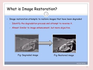
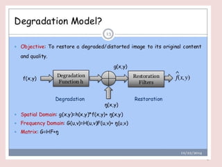
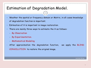
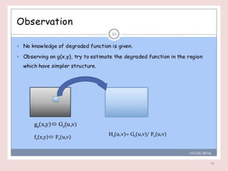
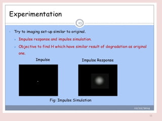
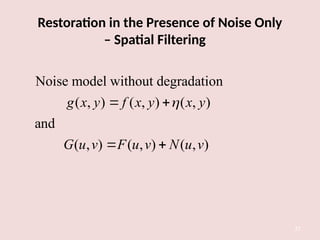
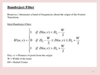
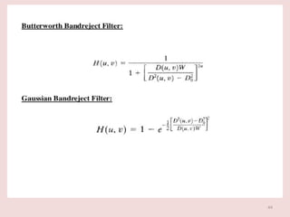
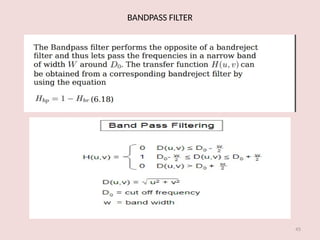
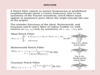
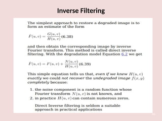
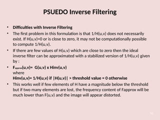
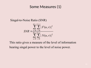
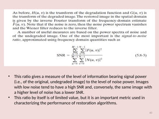
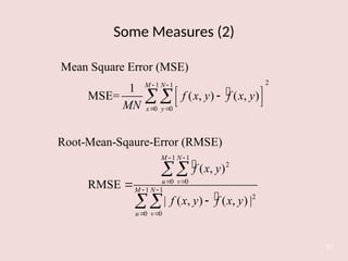
1. 1
Digital Image Processing
UNIT 3

2. 2

3. 3

4. 4

5. 5

6. Image Restoration
• Image restoration: recover an image that
has been degraded by using a prior
knowledge of the degradation
phenomenon.
• Model the degradation and applying the
inverse process in order to recover the
original image.
6

7. 7

8. 8
• As in image enhancement, the principal goal of restoration
techniques is to improve an image in some predefined sense.
• Although there are areas of overlap, image enhancement is
largely a subjective process, while image restoration is for the
most part an objective process.
• Restoration attempts to recover an image that has been
degraded by using a priori knowledge of the degradation
phenomenon.
• Thus, restoration techniques are oriented toward modeling
the degradation and applying the inverse process in order to
recover the original image.
• This approach usually involves formulating a criterion of
goodness that will yield an optimal estimate of the desired
result.

9. 9

10. 10

11. 11

12. Mathematical Modeling (1)
12
► Environmental conditions cause degradation
A model about atmospheric turbulence
2 2 5/6
( )
( , )
: a constant that depends on
the nature of the turbulence
k u v
H u v e
k
 


13. A Model of Image Degradation/Restoration
Process
13
►Degradation
 Degradation function H
 Additive noise )
,
( y
x


14. NOISE MODELS
• Image noise is random variation of brightness or color
information in images, and is usually an aspect of electronic
noise.
• It can be produced by the sensor and circuitry of
a scanner or digital camera.
• The principal sources of noise in digital images arise during
image acquisition and/or transmission
• Image acquisition
e.g., light levels, sensor temperature, etc.
• Transmission
e.g., lightning or other atmospheric disturbance in wireless
network
14

15. 15

16. 16

17. 17

18. 18

19. 19

20. 20

21. 21

22. 22

23. 23

24. 24

25. Examples of Noise: Noisy Images(2)
25

26. 26

27. Restoration in the Presence of Noise Only
̶ Spatial Filtering
27
Noise model without degradation
( , ) ( , ) ( , )
and
( , ) ( , ) ( , )
g x y f x y x y
G u v F u v N u v

 
 

28. 28

29. 29

30. 30

31. 31

32. Spatial Filtering: Mean Filters (4)
32

1
( , )
( , )
Contraharmonic mean filter
( , )
( , )
( , )
xy
xy
Q
s t S
Q
s t S
g s t
f x y
g s t






Q is the order of the filter.
It is well suited for reducing the effects of salt-and-
pepper noise. Q>0 for pepper noise and Q<0 for salt
noise.

33. 33

34. 34

35. 35

36. 36

37. 37

38. 38

39. 39

40. Periodic Noise Reduction by Frequency Domain Filtering
40

41. 41

42. 42

43. 43

44. 44

45. 45
BANDPASS FILTER

46. 46
NOTCH FILTER

47. 47

48. 48

49. Inverse Filtering
49

50. PSUEDO Inverse Filtering
• Difficulties with Inverse Filtering
• The first problem in this formulation is that 1/H(u,v) does not necessarily
exist. If H(u,v)=0 or is close to zero, it may not be computationally possible
to compute 1/H(u,v).
• If there are few values of H(u,v) which are close to zero then the ideal
inverse filter can be approximated with a stabilized version of 1/H(u,v) given
by :
• Fapprox(u,v)= G(u,v) x Hinv(u,v)
where
Hinv(u,v)= 1/H(u,v) if |H(u,v)| > threshold value = 0 otherwise
• This works well if few elements of H have a magnitude below the threshold
but if two many elements are lost, the frequency content of Fapprox will be
much lower than F(u,v) and the image will appear distorted.
50

51. 51

52. Minimum Mean Square Error (Wiener) Filtering
52
 N. Wiener (1942)
 Objective
Find an estimate of the uncorrupted image such that the mean
square error between them is minimized

 
2 2
( )
e E f f
 

53. Minimum Mean Square Error (Wiener) Filtering
53

2
2
The minimum of the error function is given in the frequency domain
by the expression
*( , ) ( , )
( , ) ( , )
( , ) | ( , ) | ( , )
*( , )
| ( , ) | ( ,
f
f
H u v S u v
F u v G u v
S u v H u v S u v
H u v
H u v S u v


 
 

 
 


2
2
( , )
) / ( , )
1 | ( , ) |
( , )
( , ) | ( , ) | ( , ) / ( , )
f
f
G u v
S u v
H u v
G u v
H u v H u v S u v S u v

 
 
 
 
 
 

 
 

54. Minimum Mean Square Error (Wiener) Filtering
54

2
2
2
2
1 | ( , ) |
( , ) ( , )
( , ) | ( , ) | ( , ) / ( , )
( , ) :degradation function
*( , ): complex conjugate of ( , )
| ( , ) | *( , ) ( , )
( , ) | ( , ) | power spectrum of the noise
( ,
f
f
H u v
F u v G u v
H u v H u v S u v S u v
H u v
H u v H u v
H u v H u v H u v
S u v N u v
S u v


 
 

 
 

 
2
) | ( , ) | power spectrum of the undegraded image
F u v
 

55. • The filter, which consists of the terms inside the
brackets, also is commonly referred to as the
minimum mean square error filter or the least square
error filter.
• Wiener filter does not have the same problem as the
inverse filter with zeros in the degradation function,
unless the entire denominator is zero for the same
value(s) of u and v.
55

56. 56

57. 57

58. Minimum Mean Square Error (Wiener) Filtering
58

2
2
1 | ( , ) |
( , ) ( , )
( , ) | ( , ) |
is a specified constant. Generally, the value of K
is chosen interactively to yield the best visual results.
H u v
F u v G u v
H u v H u v K
K
 
 

 

59. Some Measures (1)
59
1 1
2
0 0
1 1
2
0 0
Singal-to-Noise Ratio (SNR)
| ( , ) |
| ( , ) |
This ratio gives a measure of the level of information
bearing singal power to the level of noise power.
M N
u v
M N
u v
F u v
SNR
N u v
 
 
 
 




60. 60
• This ratio gives a measure of the level of information bearing signal power
(i.e., of the original, undegraded image) to the level of noise power. Images
with low noise tend to have a high SNR and, conversely, the same image with
a higher level of noise has a lower SNR.
• This ratio by itself is of limited value, but it is an important metric used in
characterizing the performance of restoration algorithms.

61. Some Measures (2)
61



2
1 1
0 0
1 1
2
0 0
1 1
2
0 0
Mean Square Error (MSE)
1
MSE= ( , ) ( , )
Root-Mean-Sqaure-Error (RMSE)
( , )
RMSE
| ( , ) ( , ) |
M N
x y
M N
u v
M N
u v
f x y f x y
MN
f x y
f x y f x y
 
 
 
 
 
 
 

 




