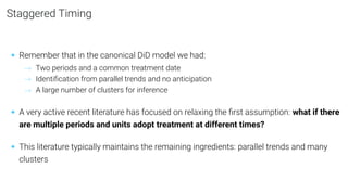
The document discusses the challenges and advancements in estimating treatment effects within staggered Treatment Effects Designs (DIDs) involving multiple periods and varying adoption times. It outlines negative results from traditional methods, highlights new estimators that aim to improve estimation accuracy, and emphasizes the importance of using clean comparisons for robust analysis. The text also offers personal advice on navigating the complexities of this recent literature and understanding its impact on empirical results.

2. Staggered Timing
• Remember that in the canonical DiD model we had:
→ Two periods and a common treatment date
→ Identification from parallel trends and no anticipation
→ A large number of clusters for inference
• A very active recent literature has focused on relaxing the first assumption: what if there
are multiple periods and units adopt treatment at different times?
• This literature typically maintains the remaining ingredients: parallel trends and many
clusters

3. Overview of Staggered Timing Literature
1. Negative results: TWFE OLS doesn’t give us what we want with treatment effect
heterogeneity
2. New estimators: perform better under treatment effect heterogeneity

4. Staggered timing set-up
• Panel of observations for periods t = 1, ..., T
• Suppose units adopt a binary treatment at different dates Gi ∈ {1, ..., T} ∪ ∞ (where
Gi = ∞ means “never-treated”)
→ Literature is now starting to consider cases with continuous treatment & treatments that turn
on/off – that lit is still developing (see Section 3.4 of review paper)
• Potential outcomes Yit(g) – depend on time and time you were first-treated

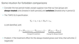
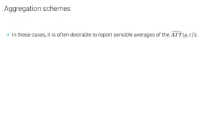
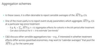
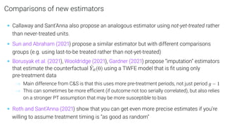
5. Extending the Identifying Assumptions
• The key identifying assumptions from the canonical model are extended in the natural way
• Parallel trends: Intuitively, says that if treatment hadn’t happened, all “adoption cohorts”
would have parallel average outcomes in all periods
E[Yit(∞) − Yi,t−1(∞)|Gi = g] = E[Yit(∞) − Yi,t−1(∞)|Gi = g0
] for all g, g0
, t, t0
Note: can impose slightly weaker versions (e.g. only require PT post-treatment)
• No anticipation: Intuitively, says that treatment has no impact before it is implemented
Yit(g) = Yit(∞) for all t < g

6. Negative results
• Suppose we again run the regression
Yit = αi + φt + Ditβ + it,
where Dit = 1[t ≥ Gi] is a treatment indicator.
• Suppose we’re willing to assume no anticipation and parallel trends across all adoption
cohorts as described above

7. Negative results
• Suppose we again run the regression
Yit = αi + φt + Ditβ + it,
where Dit = 1[t ≥ Gi] is a treatment indicator.
• Suppose we’re willing to assume no anticipation and parallel trends across all adoption
cohorts as described above
• Good news: if treatment effects are constant across time and units, Yit(g) − Yit(∞) ≡ τ,
then β = τ

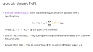
8. Negative results
• Suppose we again run the regression
Yit = αi + φt + Ditβ + it,
where Dit = 1[t ≥ Gi] is a treatment indicator.
• Suppose we’re willing to assume no anticipation and parallel trends across all adoption
cohorts as described above
• Good news: if treatment effects are constant across time and units, Yit(g) − Yit(∞) ≡ τ,
then β = τ
• Bad news: if treatment effects are not constant across time/units, then β may put
negative weights on treatment effects for some units and time periods
→ E.g., if treatment effect depends on time since treatment, Yit(t − r) − Yit(∞) = τr, then some
τrs may get negative weight

9. Where do these negative results come from?
• The intuition for these negative results is that the TWFE OLS specification combines two
sources of comparisons:
1. Clean comparisons: DiD’s between treated and not-yet-treated units
2. Forbidden comparisons: DiD’s between two sets of already-treated units (who began
treatment at different times)
• These forbidden comparisons can lead to negative weights: the “control group” is already
treated, so we run into problems if their treatment effects change over time

10. Some intuition for forbidden comparisons
• Consider the two period model, except suppose now that our two groups are
always-treated units (treated in both periods) and switchers (treated only in period 2)
• The TWFE OLS specification
Yit = αi + φt + Ditβ + it,
is still identified, with
β̂ = ȲSwitchers,2 − ȲSwitchers,1
| {z }
Change for switchers
− ȲAT,2 − ȲAT,1
| {z }
Change for always treated
• Problem: if the treatment effect for the always-treated grows over time, that will enter β̂
negatively!

11. Not just negative but weird...
The literature has placed a lot of emphasis on the fact that some treatment effects may get
negative weights
• But even if the weights are non-negative, they might not give us the most intuitive
parameter
• For example, suppose each unit i has treatment effect τi in every period if they are treated
(no dynamics). Then β gives a weighted average of the τi where the weights are largest
for units treated closest to the middle of the panel
• It is not obvious that these weights are relevant for policy, even if they are all non-negative!

12. Issues with dynamic TWFE
• Sun and Abraham (2021) show that similar issues arise with dynamic TWFE
specifications:
Yi,t = αi + λt +
X
k6=0
γkDk
i,t + εi,t,
where Dk
i,t = 1 {t − Gi = k} are “event-time” dummies.
• Like for the static spec, γk may put negative weight on treatment effects after k periods
for some units
• SA also show that γk may be “contaminated” by treatment effects at lags k0 6= k

13. Dynamic TWFE - Continued
• The results in SA suggest that interpreting the γ̂k for k = 1, 2, ... as estimates of the
dynamic effects of treatment may be misleading
• These results also imply that pre-trends tests of the γk for k 0 may be misleading –
could be non-zero even if parallel trends holds, since they may be “contaminated” by
post-treatment effects!

14. Dynamic TWFE - Continued
• The results in SA suggest that interpreting the γ̂k for k = 1, 2, ... as estimates of the
dynamic effects of treatment may be misleading
• These results also imply that pre-trends tests of the γk for k 0 may be misleading –
could be non-zero even if parallel trends holds, since they may be “contaminated” by
post-treatment effects!
• The issues discussed in SA arise if dynamic path of treatment effects is heterogeneous
across adoption cohorts
→ Biases may be less severe than for “static” specs if dynamic patterns are similar across
cohorts

15. New estimators (and estimands!)
• Several new (closely-related) estimators have been proposed to try to address these
negative weighting issues
• The key components of all of these are:
1. Be precise about the target parameter (estimand) – i.e., how do we want to aggregate
treatment effects across time/units
2. Estimate the target parameter using only “clean-comparisons”

16. Example – Callaway and Sant’Anna (2020)
• Define ATT(g, t) to be ATT in period t for units first treated at period g,
ATT(g, t) = E[Yit(g) − Yit(∞)|Gi = g]

17. Example – Callaway and Sant’Anna (2020)
• Define ATT(g, t) to be ATT in period t for units first treated at period g,
ATT(g, t) = E[Yit(g) − Yit(∞)|Gi = g]
• Under PT and No Anticipation, ATT(g, t) is identified as
ATT(g, t) = E[Yit − Yi,g−1|Gi = g]
| {z }
Change for cohort g
− E[Yit − Yi,g−1|Gi = ∞]
| {z }
Change for never-treated units
• Why?

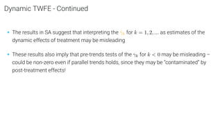
18. Example – Callaway and Sant’Anna (2020)
• Define ATT(g, t) to be ATT in period t for units first treated at period g,
ATT(g, t) = E[Yit(g) − Yit(∞)|Gi = g]
• Under PT and No Anticipation, ATT(g, t) is identified as
ATT(g, t) = E[Yit − Yi,g−1|Gi = g]
| {z }
Change for cohort g
− E[Yit − Yi,g−1|Gi = ∞]
| {z }
Change for never-treated units
• Why? This is a two-group two-period comparison, so the argument is the same as in the
canonical case!

19. Proof of Identification Argument
• Start with
E[Yit − Yi,g−1|Gi = g] − E[Yit − Yi,g−1|Gi = ∞]

20. Proof of Identification Argument
• Start with
E[Yit − Yi,g−1|Gi = g] − E[Yit − Yi,g−1|Gi = ∞]
• Apply definition of POs to obtain:
E[Yit(g) − Yi,g−1(g)|Gi = g] − E[Yig(∞) − Yi,g−1(∞)|Gi = ∞]

21. Proof of Identification Argument
• Start with
E[Yit − Yi,g−1|Gi = g] − E[Yit − Yi,g−1|Gi = ∞]
• Apply definition of POs to obtain:
E[Yit(g) − Yi,g−1(g)|Gi = g] − E[Yig(∞) − Yi,g−1(∞)|Gi = ∞]
• Use No Anticipation to substitute Yi,g−1(∞) for Yi,g−1(g):
E[Yit(g) − Yi,g−1(∞)|Gi = g] − E[Yig(∞) − Yi,g−1(∞)|Gi = ∞]

22. Proof of Identification Argument
• Start with
E[Yit − Yi,g−1|Gi = g] − E[Yit − Yi,g−1|Gi = ∞]
• Apply definition of POs to obtain:
E[Yit(g) − Yi,g−1(g)|Gi = g] − E[Yig(∞) − Yi,g−1(∞)|Gi = ∞]
• Use No Anticipation to substitute Yi,g−1(∞) for Yi,g−1(g):
E[Yit(g) − Yi,g−1(∞)|Gi = g] − E[Yig(∞) − Yi,g−1(∞)|Gi = ∞]
• Add and subtract E[Yit(∞)|Gi = g] to obtain:
E[Yit(g) − Yit(∞)|Gi = g]+
[E[Yit(∞) − Yi,g−1(∞)|Gi = g] − E[Yig(∞) − Yi,g−1(∞)|Gi = ∞]]

23. Proof of Identification Argument
• Start with
E[Yit − Yi,g−1|Gi = g] − E[Yit − Yi,g−1|Gi = ∞]
• Apply definition of POs to obtain:
E[Yit(g) − Yi,g−1(g)|Gi = g] − E[Yig(∞) − Yi,g−1(∞)|Gi = ∞]
• Use No Anticipation to substitute Yi,g−1(∞) for Yi,g−1(g):
E[Yit(g) − Yi,g−1(∞)|Gi = g] − E[Yig(∞) − Yi,g−1(∞)|Gi = ∞]
• Add and subtract E[Yit(∞)|Gi = g] to obtain:
E[Yit(g) − Yit(∞)|Gi = g]+
[E[Yit(∞) − Yi,g−1(∞)|Gi = g] − E[Yig(∞) − Yi,g−1(∞)|Gi = ∞]]
• Cancel the last term using PT to get E[Yit(g) − Yit(∞)|Gi = g] = ATT(g, t)

24. Example – Callaway and Sant’Anna (2020)
• Define ATT(g, t) to be ATT in period t for units first treated at period g,
ATT(g, t) = E[Yit(g) − Yit(∞)|Gi = g]

25. Example – Callaway and Sant’Anna (2020)
• Define ATT(g, t) to be ATT in period t for units first treated at period g,
ATT(g, t) = E[Yit(g) − Yit(∞)|Gi = g]
• Under PT and No Anticipation,
ATT(g, t) = E[Yit − Yi,g−1|Gi = g]
| {z }
Change for cohort g
− E[Yit − Yi,g−1|Gi = ∞]
| {z }
Change for never-treated

26. Example – Callaway and Sant’Anna (2020)
• Define ATT(g, t) to be ATT in period t for units first treated at period g,
ATT(g, t) = E[Yit(g) − Yit(∞)|Gi = g]
• Under PT and No Anticipation,
ATT(g, t) = E[Yit − Yi,g−1|Gi = g]
| {z }
Change for cohort g
− E[Yit − Yi,g−1|Gi = ∞]
| {z }
Change for never-treated
• We can then estimate this with sample analogs:
[
ATT(g, t) = b
E[Yit − Yi,g−1|Gi = g]
| {z }
Sample change for cohort g
− b
E[Yit − Yi,g−1|Gi = ∞]
| {z }
Sample change for never-treated
where Ê denotes sample means.

27. Aggregation schemes
• If have a large number of observations and relatively few groups/periods, can report
[
ATT(g, t)’s directly.
• If there are many groups/periods, the [
ATT(g, t) may be very imprecisely estimated
and/or too numerous to report concisely

28. Aggregation schemes
• In these cases, it is often desirable to report sensible averages of the [
ATT(g, t)’s.

29. Aggregation schemes
• In these cases, it is often desirable to report sensible averages of the [
ATT(g, t)’s.
• One of the most useful is to report event-study parameters which aggregate [
ATT(g, t)’s
at a particular lag since treatment
→ E.g. θ̂k =
P
g
[
ATT(g, t + k) aggregates effects for cohorts in the kth period after treatment
→ Can also construct for k 0 to estimate “pre-trends”

30. Aggregation schemes
• In these cases, it is often desirable to report sensible averages of the [
ATT(g, t)’s.
• One of the most useful is to report event-study parameters which aggregate [
ATT(g, t)’s
at a particular lag since treatment
→ E.g. θ̂k =
P
g
[
ATT(g, t + k) aggregates effects for cohorts in the kth period after treatment
→ Can also construct for k 0 to estimate “pre-trends”
• CS discuss other sensible aggregations too – e.g., if interested in whether treatment
effects differ across good/bad economies, may want to “calendar averages” that pool the
[
ATT(t, g) for the same year

31. Comparisons of new estimators
• Callaway and Sant’Anna also propose an analogous estimator using not-yet-treated rather
than never-treated units.
• Sun and Abraham (2021) propose a similar estimator but with different comparisons
groups (e.g. using last-to-be treated rather than not-yet-treated)
• Borusyak et al. (2021), Wooldridge (2021), Gardner (2021) propose “imputation” estimators
that estimate the counterfactual Ŷit(0) using a TWFE model that is fit using only
pre-treatment data
→ Main difference from CS is that this uses more pre-treatment periods, not just period g − 1
→ This can sometimes be more efficient (if outcome not too serially correlated), but also relies
on a stronger PT assumption that may be more susceptible to bias
• Roth and Sant’Anna (2021) show that you can get even more precise estimates if you’re
willing to assume treatment timing is “as good as random”

32. Personal advice
• Don’t freak out about this new literature!

33. Personal advice
• Don’t freak out about this new literature!
• In most cases, using the “new” DiD methods will not lead to a big change in your results
(empirically, TE heterogeneity is not that large in most cases)
→ The exceptions are cases where there are many periods with very few treated units – this is
when “forbidden comparisons” get the most weight

34. Personal advice
• Don’t freak out about this new literature!
• In most cases, using the “new” DiD methods will not lead to a big change in your results
(empirically, TE heterogeneity is not that large in most cases)
→ The exceptions are cases where there are many periods with very few treated units – this is
when “forbidden comparisons” get the most weight
• The most important thing is to be precise about who you want the comparison group to
be and to choose a method that only uses these “clean comparisons”

35. Personal advice
• Don’t freak out about this new literature!
• In most cases, using the “new” DiD methods will not lead to a big change in your results
(empirically, TE heterogeneity is not that large in most cases)
→ The exceptions are cases where there are many periods with very few treated units – this is
when “forbidden comparisons” get the most weight
• The most important thing is to be precise about who you want the comparison group to
be and to choose a method that only uses these “clean comparisons”
• In my experience, the difference between the new estimators is typically not that large –
can report multiple new methods for robustness (to make your referees happy!)

36. References I
Borusyak, Kirill, Xavier Jaravel, and Jann Spiess, “Revisiting Event Study Designs: Robust
and Efficient Estimation,” arXiv:2108.12419 [econ], 2021.
Gardner, John, “Two-stage differences in differences,” Working Paper, 2021.
Roth, Jonathan and Pedro H. C. Sant’Anna, “Efficient Estimation for Staggered Rollout
Designs,” arXiv:2102.01291 [econ, math, stat], 2021.
Sun, Liyang and Sarah Abraham, “Estimating dynamic treatment effects in event studies
with heterogeneous treatment effects,” Journal of Econometrics, 2021, 225 (2), 175–199.
Wooldridge, Jeffrey M, “Two-Way Fixed Effects, the Two-Way Mundlak Regression, and
Difference-in-Differences Estimators,” Working Paper, 2021, pp. 1–89.