The document discusses machine learning concepts, focusing on conditional probability, Bayes' theorem, and various algorithms like Naïve Bayes and K-Nearest Neighbors (KNN). It explains the calculations of probabilities in the context of health-related tests and how to classify data based on user ratings for recommendation systems. The text also covers filtering methods for recommendations, including collaborative and content filtering, along with the challenges faced in implementing these systems.

![Bayes Theorem
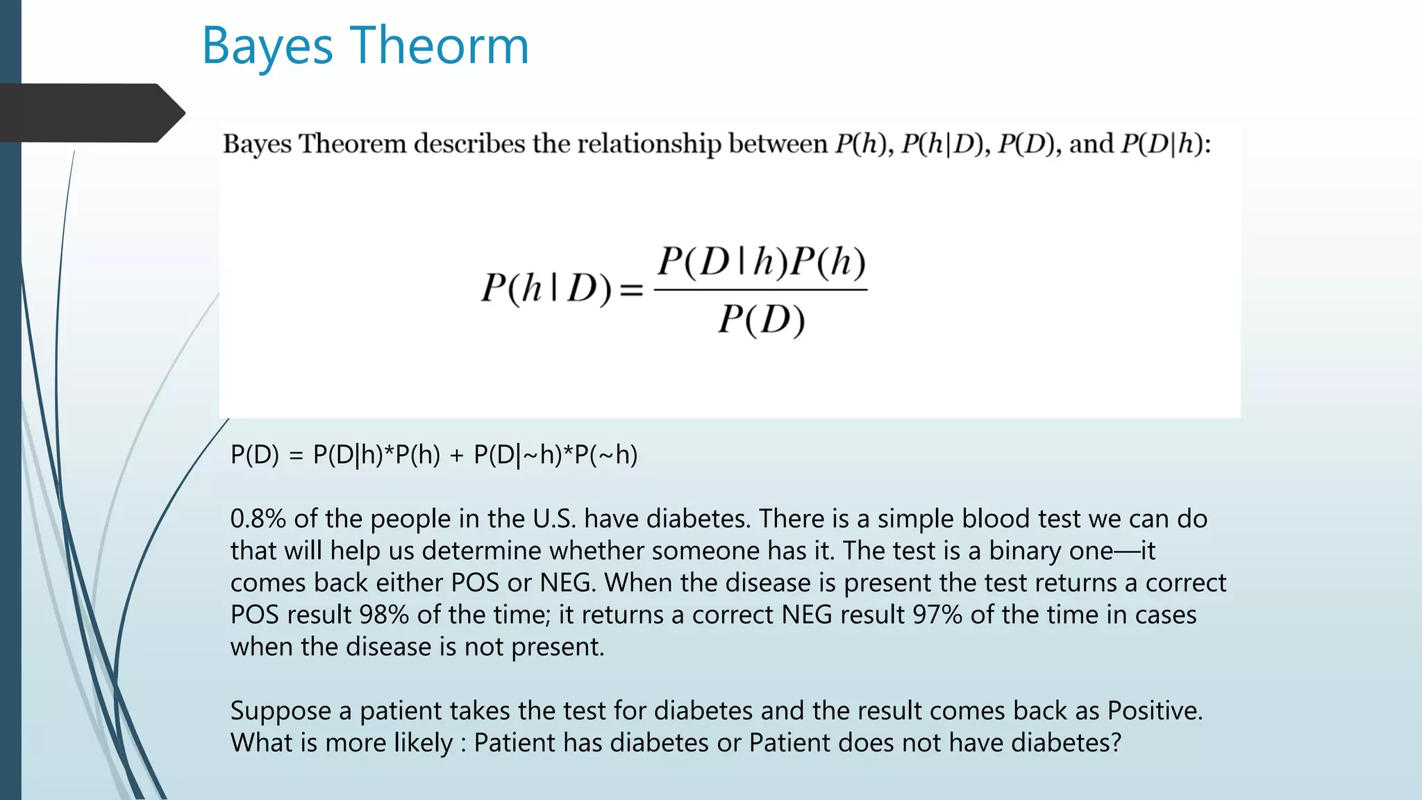
P(disease) = 0.008
P(~disease) = 0.992
P(POS|disease) = 0.98
P(NEG|disease) = 0.02
P(NEG|~disease)=0.97
P(POS|~disease) = 0.03
P(disease|POS) = ??
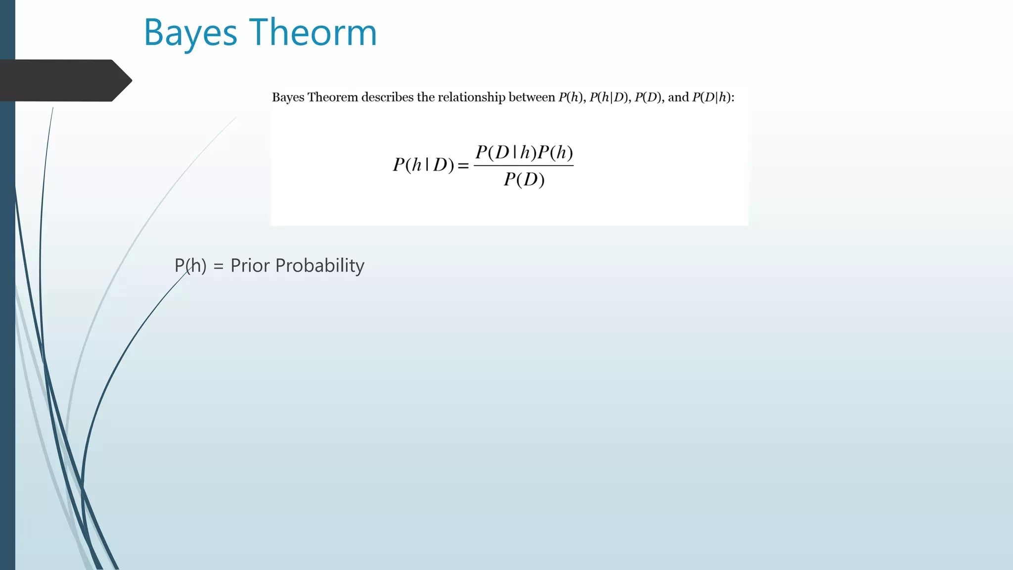
As per Bayes Theorm:
P(disease|POS) = [P(POS|disease)* P(disease)]/P(POS)
P(POS) = P(POS|disease)* P(disease)] + P(POS|~disease)* P(~disease)]
P(disease|POS) = 0.98*0.008/(0.98*0.008 + 0.03*0.992) = 0.21
P(~disease|POS) = 0.03*0.992/(0.98*0.008 + 0.03*0.992) = 0.79
The person has only 21% chance of getting the disease](https://image.slidesharecdn.com/machinelearning-session7nbclassifierknn-180915175536/75/Machine-learning-session7-nb-classifier-k-nn-7-2048.jpg)