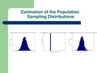
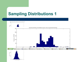
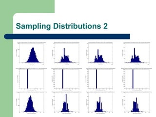
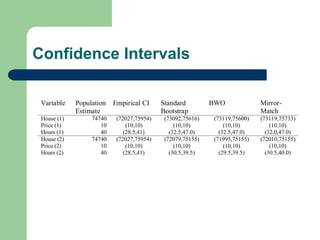
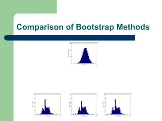
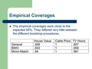
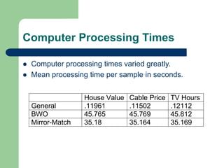
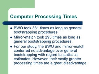
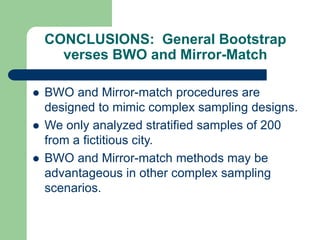
This document describes a bootstrap project analyzing population and sampling distributions using different bootstrap methods. It summarizes the general bootstrap method, bootstrap without replacement (BWO), and mirror-match approaches. Results show the bootstrap sampling distributions mimic the actual distributions and produce accurate estimates of statistics and variances. However, BWO and mirror-match had vastly greater processing times with no statistical advantage over the general bootstrap method for the stratified samples analyzed in this study.

1. STAT 572: Bootstrap Project
Group Members:
Cindy Bothwell
Erik Barry Erhardt
Nina Greenberg
Casey Richardson
Zachary Taylor

2. Histograms of Complex Population
Distribution

3. Histograms of Population Sampling
Distribution of the Median and Estimated
Bootstrap Sampling Distributions

4. What is a Bootstrap
 A method of Resampling: creating many
samples from a single sample
 Generally, resampling is done with
replacement
 Used to develop a sampling distribution of
statistics such as mean, median, proportion,
others.

5. The Bootstrap and Complex Surveys
 Number of bootstrap samples
– n = sample size, N = population size
– Possible resamples nn (example n=200,
200200=1.6x10460)
 Too many possibilities N!/[n!(N-n)!], limit to B a
large number, (example = 1000) - the Monte
Carlo approximation
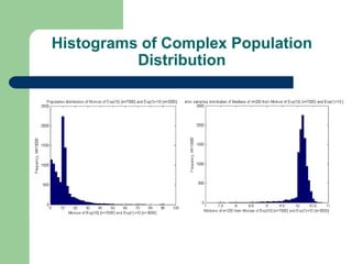
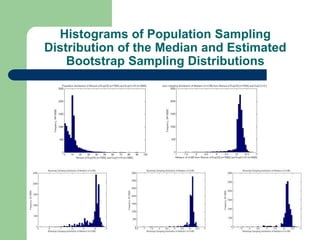
 Determine sampling distribution with parameters
 Calculate variance in the normal way

6. Advantages and Disadvantages
 Advantages:
– Avoids the costs of taking new samples (Estimate a
sampling distribution when only one sample is available)
– Checking parametric assumptions
– Used when parametric assumptions cannot be made or are
very complicated
– Estimation of variance in quantiles
 Disadvantages:
– Relies on a representative sample
– Variability due to finite replications (Monte Carlo)

7. Computations
 With more computing power available, bootstrap is
possible for a large number of resamples
 Possible programs:
– Matlab
– Minitab
– SAS
– Excel
– S-Plus
– SPSS
– Fathom

8. Bootstrap using SURVEY program
 Main parameter of interest is the median price that
all households in Lockhart City are wiling to pay for
cable.
 The price that a household is willing to pay for cable
is positively correlated with average-district house
value.
 Districts in Lockhart City are divided into strata
based on average house value.
 Estimate the variance and create 95% CI

9. Lockhart City Strata Characteristics:
 Take a stratified
random sample of size
200 using proportional
allocation.
 Using the stratified
random sample,
implement the general
bootstrap procedure,
BWO, and mirror-
match.
Stratum Districts
House Value
($1,000) N n
1 53, 54, 55, 59, 60 35-55 3529 36
2 52, 58, 63, 64, 65 55-70 4775 49
3 62, 68, 69, 70, 73 70-80 4257 43
4 57, 67, 72, 74, 75 80-85 4077 41
5 51, 56, 61, 66, 71 85-105 3026 31
Table 1: Lockhart City Stratum based on House Value

10. Variations of the Bootstrap in Strata
 General Bootstrap
– Mimic the original sampling method
 BWO: Bootstrap Without Replacement
– Grow the sample to the size of the population
 Mirror-Match
– Repeated miniature resamples

11. BWO: Bootstrap Without Replacement
 Grow the sample to the size of the population
 For each stratum L, create a pseudo-
population by replicating the sample kL times.
 Resample n’L units from each stratum without
replacement to obtain a single bootstrap
sample for stratum L.
 Repeat a large number of times

12. BWO: Variable Definitions
 
L
L
L f
n
n 

 1
' where
L
L
L
N
n
f  = stratum sampling fraction
 







 


L
L
L
L
L
n
f
n
N
k
1
1 where L
n' and L
k are integers

13. Disadvantages of extended BWO
 NL must be known
 n’L and kL are often non-integers
 Must bracket between integers if n’L and kL
are non-integer
 Computing time

14. Mirror-Match
 Repeated miniature resamples
 Resample size is determined to match the proportion
of the original sample size to the population sample
size (nL/NL).
 Using the resample size n’L, we resample n’L units
(SRSWOR) from each stratum L.
 Repeat previous step kL times with replacement to
obtain a single bootstrap sample for stratum L.
 Repeat a large number times

15. Mirror-Match: Variable Definitions
L
L
L
N
n
n
2
' 
 
 
L
L
L
L
L
f
n
f
n
k



1
'
*
1
where:
L
L
L
n
n
f
'
*  = stratum resample fraction
L
L
L
N
n
f  = original stratum sample fraction

16. Mirror Match: Disadvantages
 NL must be known
 kL is often non-integer
 Must bracket between integers when kL is
non-integer
 Computing time

17. Estimation of the Population
Sampling Distributions
 100,000 independent stratified random
samples.
 Medians computed and plotted to form
empirical sampling distributions.
 Variables: house value, cable price, and TV
hours.

18. Estimation of the Population
Sampling Distributions

19. Simulations
 Matlab code: General, BWO, and Mirror-match.
 Two independent stratified random samples from
Lockhart City.
 Comparison of the sample bootstrap sampling
distributions with the population sampling
distributions.
 95% confidence intervals were determined bootstrap
2.5 and 97.5 percentiles.

20. Sampling Distributions 1

21. Sampling Distributions 2

22. Confidence Intervals
Variable Population
Estimate
Empirical CI Standard
Bootstrap
BWO Mirror-
Match
House (1) 74740 (72027,75954) (73092,75616) (73119,75600) (73119,75733)
Price (1) 10 (10,10) (10,10) (10,10) (10,10)
Hours (1) 40 (28.5,41) (32.5,47.0) (32.5,47.0) (32.0,47.0)
House (2) 74740 (72027,75954) (72079,75155) (71995,75155) (72010,75155)
Price (2) 10 (10,10) (10,10) (10,10) (10,10)
Hours (2) 40 (28.5,41) (30.5,39.5) (29.5,39.5) (30.5,40.0)

23. The Empirical verses the Bootstrap
Sampling Distributions
 Bootstrap sampling distributions are expected to
mimic actual sampling distributions.
 Bootstrap sampling is sensitive to individual samples.
 The shape of bootstrap sampling distributions may
vary, but the statistic of interest and its variance are
considered accurate.

24. Comparison of Bootstrap Methods

25. Empirical Coverages
 The empirical coverages were close to the
expected 95%. They differed very little between
the different bootstrap procedures.
House Value Cable Price TV Hours
General .936 1 .957
BWO .933 1 .959
Mirror-Match .94 1 .961

26. Empirical Coverages
 Empirical coverages are dependent on the type of
confidence interval that was originally selected.
 Our confidence intervals were calculated from the
2.5 and 97.5 percentiles of each bootstrap
distribution.
 There are many different types of bootstrap
confidence intervals. The one we selected, although
intuitive in design, is considered generally biased
(Bedrick 2006).

27. Computer Processing Times
 Computer processing times varied greatly.
 Mean processing time per sample in seconds.
House Value Cable Price TV Hours
General .11961 .11502 .12112
BWO 45.765 45.769 45.812
Mirror-Match 35.18 35.164 35.169

28. Computer Processing Times
 BWO took 381 times as long as general
bootstrapping procedures.
 Mirror-match took 293 times as long as
general bootstrapping procedures.
 For our study, the BWO and mirror-match
conferred no advantage over general
bootstrapping with regard to statistical
estimates. However, their vastly greater
processing times are a great disadvantage.

29. CONCLUSIONS: General Bootstrap
verses BWO and Mirror-Match
 BWO and Mirror-match procedures are
designed to mimic complex sampling designs.
 We only analyzed stratified samples of 200
from a fictitious city.
 BWO and Mirror-match methods may be
advantageous in other complex sampling
scenarios.