This document provides an overview of key concepts in statistics, machine learning, and data science. It discusses topics such as populations and samples, parameters and statistics, measures of central tendency and variation, hypothesis testing, linear and logistic regression, decision trees, overfitting and regularization, bagging and boosting, and random forests. The document also provides examples to illustrate statistical fundamentals like hypothesis testing, one sample t-tests, and type I and II errors.

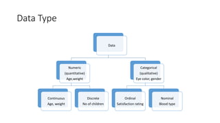
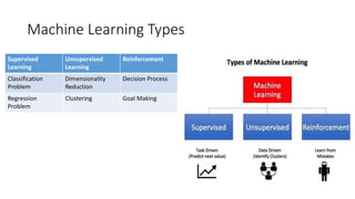
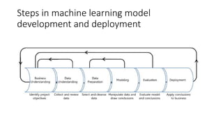
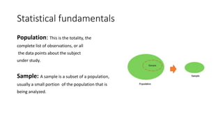
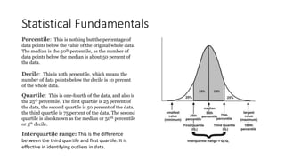
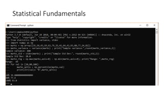
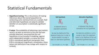
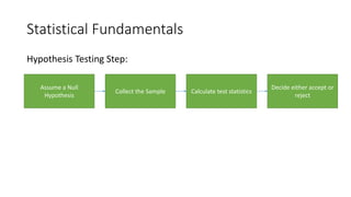
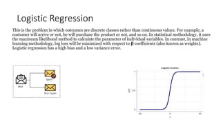
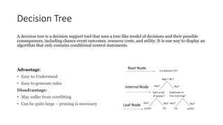
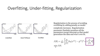
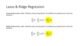
2. Bringing statistics into data science

3. Common terminology
Population Sample Probability False positives Statistical
inference Regression Fitting Categorical data Classification
Clustering Statistical comparison Coding Distributions
Data mining Decision trees Machine learning Munging and
wrangling Visualization D3 Regularization Assessment Cross-
validation Neural networks Boosting Lift Mode Outlier
Predictive modeling Big data Confidence interval Writing

4. Data Science Landscape

5. Transitioning from Data Developer to Data
Scientist

6. Data Type
Data
Numeric
(quantitative)
Age,weight
Continuous
Age, weight
Discrete
No of children
Categorical
(qualitative)
Eye color, gender
Ordinal
Satisfaction rating
Nominal
Blood type

7. Machine Learning Types
Supervised
Learning
Unsupervised
Learning
Reinforcement
Classification
Problem
Dimensionality
Reduction
Decision Process
Regression
Problem
Clustering Goal Making

8. Steps in machine learning model
development and deployment

9. Statistical fundamentals
Population: This is the totality, the
complete list of observations, or all
the data points about the subject
under study.
Sample: A sample is a subset of a population,
usually a small portion of the population that is
being analyzed.

10. Statistical fundamentals
Parameter versus statistic: Any measure that
is calculated on the population is a parameter,
whereas on a sample it is called a statistic.
Mean: This is a simple arithmetic average, which
is computed by taking the aggregated sum of
values divided by a count of those values.
Median: This is the midpoint of the data, and is
calculated by either arranging it in ascending or
descending order. If there are N observations.
Mode: This is the most repetitive data point in
the data.
Outlier: An outlier is the value of a set or
column that is highly deviant from the many other
values in the same data; it usually has very high or
low values.

11. Statistical Fundamentals

12. Statistical Fundamentals
Measure of Variation: Dispersion is the variation in the data, and measures the inconsistencies in
the value of variables in the data. Dispersion actually provides an idea about the spread rather than
central values.
Range: This is the difference between maximum & minimum of the value.
Variance: This is the mean of squared deviations from the mean (xi = data points, μ = mean of the
data, N = number of data points). The dimension of variance is the square of the actual values. The
reason to use denominator N-1 for a sample instead of N in the population is due the degree of
freedom. 1 degree of freedom lost in a sample by the time of calculating variance is due to extraction of
substitution of sample:
Standard deviation: This is the square root of variance. By applying the square root on variance, we
measure the dispersion with respect to the original variable rather than square of the dimension:
Quantile: This is the square root of variance. By applying the square root on variance, we measure the
dispersion with respect to the original variable rather than square of the dimension:

13. Statistical Fundamentals

14. Statistical Fundamentals
Percentile: This is nothing but the percentage of
data points below the value of the original whole data.
The median is the 50th percentile, as the number of
data points below the median is about 50 percent of
the data.
Decile: This is 10th percentile, which means the
number of data points below the decile is 10 percent
of the whole data.
Quartile: This is one-fourth of the data, and also is
the 25th percentile. The first quartile is 25 percent of
the data, the second quartile is 50 percent of the data,
the third quartile is 75 percent of the data. The second
quartile is also known as the median or 50th percentile
or 5th decile.
Interquartile range: This is the difference
between the third quartile and first quartile. It is
effective in identifying outliers in data.

15. Statistical Fundamentals

16. Statistical Fundamentals
• Hypothesis testing: This is the process of making
inferences about the overall population by
conducting some statistical tests on a sample. Null
and alternate hypotheses are ways to validate
whether an assumption is statistically significant
or not.
• P-value: The probability of obtaining a test statistic
result is at least as extreme as the one that was
actually observed, assuming that the null
hypothesis is true (usually in modeling, against
each independent variable, a p-value less than
0.05 is considered significant and greater than
0.05 is considered insignificant; nonetheless, these
values and definitions may change with respect to
context).

17. Statistical Fundamentals
Hypothesis Testing Step:
Assume a Null
Hypothesis
Collect the Sample Calculate test statistics
Decide either accept or
reject

18. Example of Hypothesis Testing
A chocolate manufacturer who is also your friend claims that all chocolates
produced from his factory weigh at least 1,000 g and you have got a funny
feeling that it might not be true; you both collected a sample of 30 chocolates
and found that the average chocolate weight as 990 g with sample standard
deviation as 12.5 g. Given the 0.05 significance level, can we reject the claim
made by your friend?
The null hypothesis is that μ0 ≥ 1000 (all chocolates weigh more than 1,000 g).

19. t-table

20. Example of Hypothesis Testing

21. Example of Hypothesis Testing

22. One Sample t-test
In the population the average IQ is 100. A team of scientist wants to
test a new medication to see if it has a positive or negative effect on
intelligence or no effect at all. A sample of 30 participants who have
taken the medication has a mean of 140 with SD of 20. Did the
medication affect intelligence? Alpha=0.05

23. One Sample t-test
Null & Alternative Hypothesis:
H0; u = 100
H1; u != 100
t= (xbar - u) / (s/sqrt(n))
Xbar=140 t=10.96
U=100 reject null hypothesis
S=20
N=30

24. Statistical Fundamentals
Type I and II error: Hypothesis testing is usually done on the samples rather than the entire
population, due to the practical constraints of available resources to collect all the available data.
However, performing inferences about the population from samples comes with its own costs, such as
rejecting good results or accepting false results, not to mention separately, when increases in sample
size lead to minimizing type I and II errors:
Type I Error: Rejecting a null hypothesis
when it is true
Type II Error: Accepting null hypothesis
when it is false

25. This is used for the prediction of continuous variables such as customer income and so on. It utilizes error
minimization to fit the best possible line in statistical methodology. However, in machine learning
methodology, squared loss will be minimized with respect to β coefficients. Linear regression also has a high
bias and a low variance error.
Linear Regression

26. Logistic Regression
This is the problem in which outcomes are discrete classes rather than continuous values. For example, a
customer will arrive or not, he will purchase the product or not, and so on. In statistical methodology, it uses
the maximum likelihood method to calculate the parameter of individual variables. In contrast, in machine
learning methodology, log loss will be minimized with respect to β coefficients (also known as weights).
Logistic regression has a high bias and a low variance error.

27. Decision Tree
A decision tree is a decision support tool that uses a tree-like model of decisions and their possible
consequences, including chance event outcomes, resource costs, and utility. It is one way to display an
algorithm that only contains conditional control statements.
Root Node
Internal Node
Leaf Node
Advantage:
• Easy to Understand
• Easy to generate rules
Disadvantage:
• May suffer from overfitting
• Can be quite large – pruning is necessary

28. Overfitting, Under-fitting, Regularization
Regularization is the process of avoiding
overfitting by adding penalty as model
complexity increases. Regularization
parameter (lambda) penalizes all the
parameters except intercept so that model
generalizes the data and won’t over fit.

29. Lasso & Ridge Regression
Lasso Regression: adds “absolute value of magnitude” of coefficient as penalty term to the loss
function.
Ridge Regression: adds “absolute value of magnitude” of coefficient as penalty term to the loss
function.

30. Bagging & Boosting
Boosting: This is a sequential algorithm that
applies on weak classifiers such as a decision stump
(a one-level decision tree or a tree with one root
node and two terminal nodes) to create a strong
classifier by ensembling the results. The algorithm
starts with equal weights assigned to all the
observations, followed by subsequent iterations
where more focus was given to misclassified
observations by increasing the weight of
misclassified observations and decreasing the weight
of properly classified observations. In the end, all the
individual classifiers were combined to create a
strong classifier. Boosting might have an overfitting
problem, but by carefully tuning the parameters, we
can obtain the best of the self machine learning
model.
Bagging: This is an ensemble technique applied
on decision trees in order to minimize the
variance error and at the same time not increase
the error component due to bias. In bagging,
various samples are selected with a subsample of
observations and all variables (columns),
subsequently fit individual decision trees
independently on each sample and later
ensemble the results by taking the maximum
vote (in regression cases, the mean of outcomes
calculated).

31. Bagging Boosting

32. Random Forest
Random Forest: This is similar to bagging except for one difference. In bagging, all the
variables/columns are selected for each sample, whereas in random forest a few sub columns are
selected. The reason behind the selection of a few variables rather than all was that during each
independent tree sampled, significant variables always came first in the top layer of splitting which
makes all the trees look more or less similar and defies the sole purpose of ensemble: that it works
better on diversified and independent individual models rather than correlated individual models.
Random forest has both low bias and variance errors.

33. Support vector machines (SVM)
Support vector machines (SVMs): This maximizes the margin between classes by fitting the
widest possible hyperplane between them. In the case of non-linearly separable classes, it uses kernels
to move observations into higher-dimensional space and then separates them linearly with the
hyperplane there.

34. Principal Component Analysis
Feature Extraction: Say we have ten independent variables. In feature extraction, we create ten
“new” independent variables, where each “new” independent variable is a combination of each of the
ten “old” independent variables. However, we create these new independent variables in a specific way
and order these new variables by how well they predict our dependent variable.
Principal Component Analysis: This is a dimensionality reduction technique in which principal
components are calculated in place of the original variable. Principal components are determined
where the variance in data is maximum; subsequently, the top n components will be taken by covering
about 80 percent of variance and will be used in further modeling processes, or exploratory analysis
will be performed as unsupervised learning.
Feature Elimination: Dropping Variables

35. K-means clustering:
K-means clustering: This is an unsupervised algorithm that is mainly utilized for segmentation
exercise. K-means clustering classifies the given data into k clusters in such a way that, within the
cluster, variation is minimal and across the cluster, variation is maximal.

37. Thank You