Downloaded 64 times


![Bubble Sort Implementation
Here is an ascending-order implementation of the bubblesort algorithm for integer arrays:
void BubbleSort(int List[] , int Size) {
int tempInt; // temp variable for swapping list elems
for (int Stop = Size - 1; Stop > 0; Stop--) {
for (int Check = 0; Check < Stop; Check++) { // make a pass
if (List[Check] > List[Check + 1]) { // compare elems
tempInt = List[Check]; // swap if in the
List[Check] = List[Check + 1]; // wrong order
List[Check + 1] = tempInt;
}
}
}
}
Bubblesort compares and swaps adjacent elements; simple but not very efficient.
Efficiency note: the outer loop could be modified to exit if the list is already sorted.](https://image.slidesharecdn.com/bioinformatics-t4-alignmentsv2014-141020123044-conversion-gate02/85/Bioinformatics-t4-alignments-v2014-26-320.jpg)


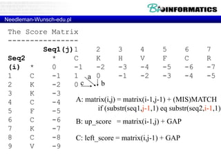
![Needleman-Wunsch.pl
# initialization
my @matrix;
$matrix[0][0]{score} = 0;
$matrix[0][0]{pointer} = "none";
for(my $j = 1; $j <= length($seq1); $j++) {
$matrix[0][$j]{score} = $GAP * $j;
$matrix[0][$j]{pointer} = "left";
}
for (my $i = 1; $i <= length($seq2); $i++) {
$matrix[$i][0]{score} = $GAP * $i;
$matrix[$i][0]{pointer} = "up";
}](https://image.slidesharecdn.com/bioinformatics-t4-alignmentsv2014-141020123044-conversion-gate02/85/Bioinformatics-t4-alignments-v2014-82-320.jpg)
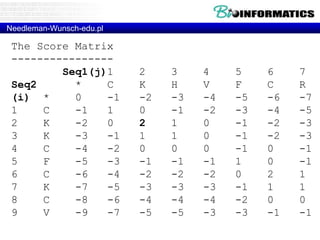
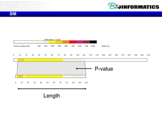
![Needleman-Wunsch.pl
# fill
for(my $i = 1; $i <= length($seq2); $i++) {
for(my $j = 1; $j <= length($seq1); $j++) {
my ($diagonal_score, $left_score, $up_score);
# calculate match score
my $letter1 = substr($seq1, $j-1, 1);
my $letter2 = substr($seq2, $i-1, 1);
if ($letter1 eq $letter2) {
$diagonal_score = $matrix[$i-1][$j-1]{score} + $MATCH;
}
else {
$diagonal_score = $matrix[$i-1][$j-1]{score} + $MISMATCH;
}
# calculate gap scores
$up_score = $matrix[$i-1][$j]{score} + $GAP;
$left_score = $matrix[$i][$j-1]{score} + $GAP;
# choose best score
if ($diagonal_score >= $up_score) {
if ($diagonal_score >= $left_score) {
$matrix[$i][$j]{score} = $diagonal_score;
$matrix[$i][$j]{pointer} = "diagonal";
}
else {
$matrix[$i][$j]{score} = $left_score;
$matrix[$i][$j]{pointer} = "left";
}
} else {
if ($up_score >= $left_score) {
$matrix[$i][$j]{score} = $up_score;
$matrix[$i][$j]{pointer} = "up";
}
else {
$matrix[$i][$j]{score} = $left_score;
$matrix[$i][$j]{pointer} = "left";
}
}](https://image.slidesharecdn.com/bioinformatics-t4-alignmentsv2014-141020123044-conversion-gate02/85/Bioinformatics-t4-alignments-v2014-85-320.jpg)
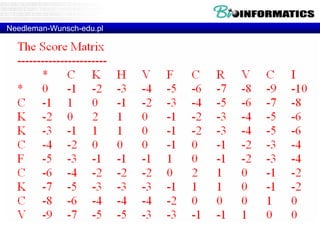
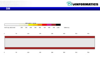
![Needleman-Wunsch.pl
my $align1 = "";
my $align2 = "";
my $j = length($seq1);
my $i = length($seq2);
while (1) {
last if $matrix[$i][$j]{pointer} eq "none";
if ($matrix[$i][$j]{pointer} eq "diagonal") {
$align1 .= substr($seq1, $j-1, 1);
$align2 .= substr($seq2, $i-1, 1);
$i--; $j--;
}
elsif ($matrix[$i][$j]{pointer} eq "left") {
$align1 .= substr($seq1, $j-1, 1);
$align2 .= "-";
$j--;
}
elsif ($matrix[$i][$j]{pointer} eq "up") {
$align1 .= "-";
$align2 .= substr($seq2, $i-1, 1);
$i--;
}
}
$align1 = reverse $align1;
$align2 = reverse $align2;
print "$align1n";
print "$align2n";](https://image.slidesharecdn.com/bioinformatics-t4-alignmentsv2014-141020123044-conversion-gate02/85/Bioinformatics-t4-alignments-v2014-90-320.jpg)
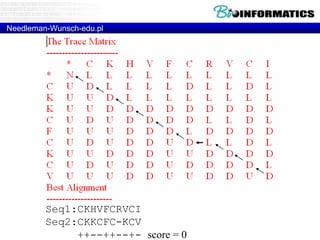

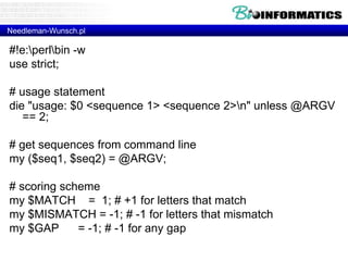
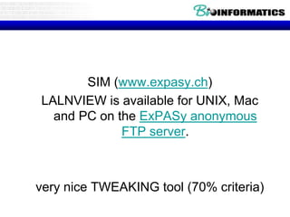
![Running ClustalW
****** MULTIPLE ALIGNMENT MENU ******
1. Do complete multiple alignment now (Slow/Accurate)
2. Produce guide tree file only
3. Do alignment using old guide tree file
4. Toggle Slow/Fast pairwise alignments = SLOW
5. Pairwise alignment parameters
6. Multiple alignment parameters
7. Reset gaps between alignments? = OFF
8. Toggle screen display = ON
9. Output format options
S. Execute a system command
H. HELP
or press [RETURN] to go back to main menu
Your choice:](https://image.slidesharecdn.com/bioinformatics-t4-alignmentsv2014-141020123044-conversion-gate02/85/Bioinformatics-t4-alignments-v2014-111-320.jpg)


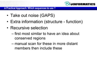

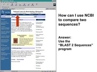
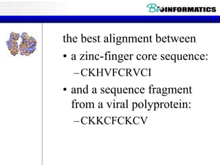
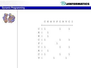
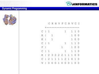
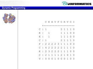
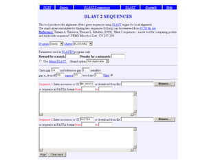
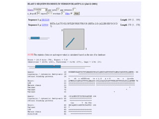
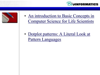
![Practical guide to pairwise alignment:
the “BLAST 2 sequences” website
• Go to http://www.ncbi.nlm.nih.gov/BLAST
• Choose BLAST 2 sequences
• In the program,
[1] choose blastp (protein search) or blastn (for DNA)
[2] paste in your accession numbers
(or use FASTA format)
[3] select optional parameters, such as
--BLOSU62 matrix is default for proteins
try PAM250 for distantly related proteins
--gap creation and extension penalties
[4] click “align”](https://image.slidesharecdn.com/bioinformatics-t4-alignmentsv2014-141020123044-conversion-gate02/85/Bioinformatics-t4-alignments-v2014-128-320.jpg)
![Practicum 3
• CpG Islands
– Download from ENSEMBL 1000 (random) promoters (3000 bp) (hint:
use Biomart)
– How many times would you expect to observe CG if all nucleotides
were equipropable
– Count the number op times CG is observed for these 1000 genes and
make a histogram from these scores.
– Are there any other dinucleatides over- or underrepresented
– CG repeats are often methylated. In order to study methylation
patterns bisulfide treatment of DNA is used. Bisulfide changes every C
which is not followed by G into T. Generate computationally the
bisulfide treated version of DNA (hint: while (s/C([^G])/T$1/g) {};)
– How would you find primers that discriminate between methylated and
unmethylated DNA ? Given that the genome is 3.109 bp how long do
you need to make a primer to avoid mispriming ?](https://image.slidesharecdn.com/bioinformatics-t4-alignmentsv2014-141020123044-conversion-gate02/85/Bioinformatics-t4-alignments-v2014-135-320.jpg)

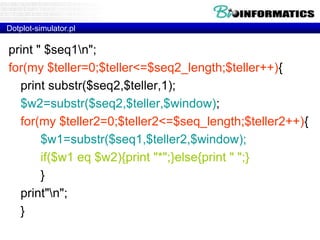
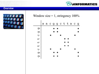
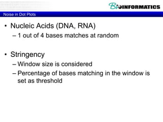
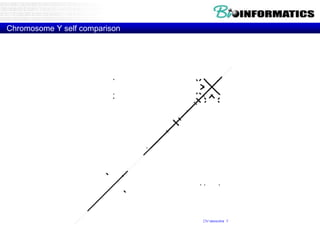
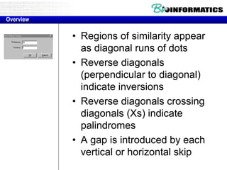
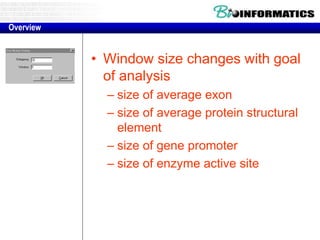
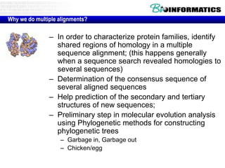
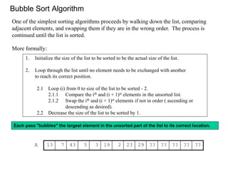
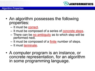
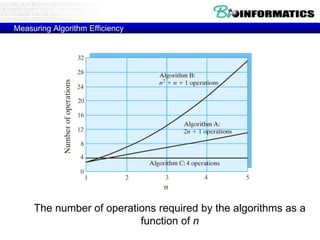
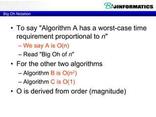
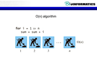
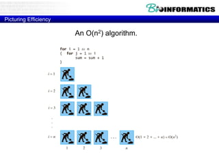
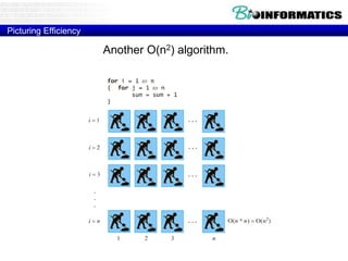
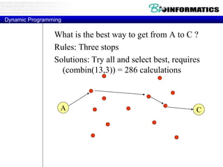
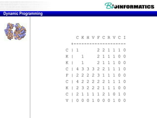
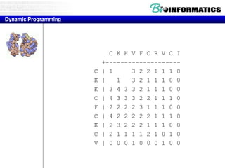
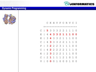
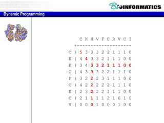
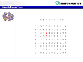
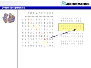
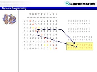
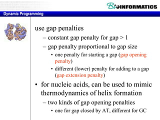
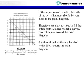
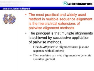
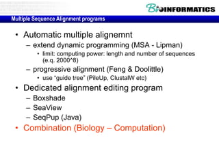
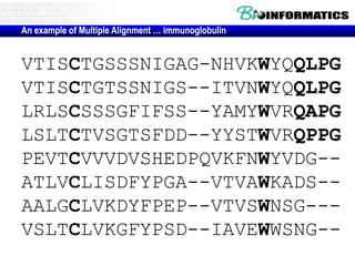
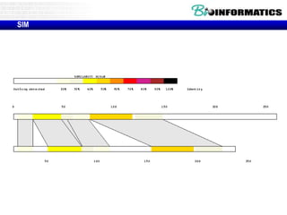
This document discusses dot plots and sequence alignments. It begins with an overview of dot plots, explaining that they are a graphical representation used to visualize similarities between two sequences. It describes how dot plots are constructed and notes that they are useful for finding repeated or inverted repeated structures. The document then discusses how to reduce noise in dot plots and provides examples of dot plots. It also discusses sequence alignments, including global vs local alignments and different algorithms for pairwise and multiple sequence alignment such as Needleman-Wunsch, Smith-Waterman, and ClustalW. It notes why multiple alignments are performed and concludes with discussing how to measure algorithm efficiency.


![Bio ontologies and semantic technologies[2]](https://cdn.slidesharecdn.com/ss_thumbnails/bioontologiesandsemantictechnologies2-180509123734-thumbnail.jpg?width=640&height=640&fit=bounds)


