The presentation introduces group members and discusses Bézier and Hermite curves. It explains the formulation and properties of both types of curves, including how they are defined by control points, their polynomials, and methods for calculating points on these curves. Additionally, the document highlights design techniques and key characteristics of Bézier curves.

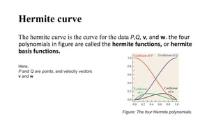
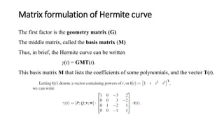
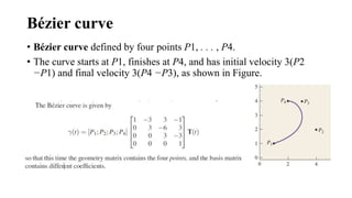
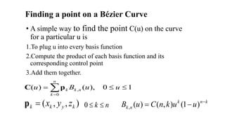
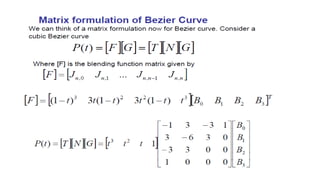
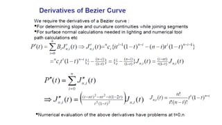
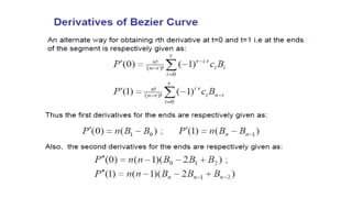
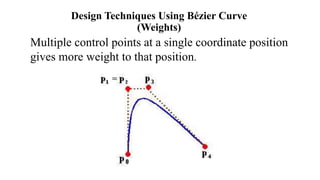
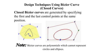
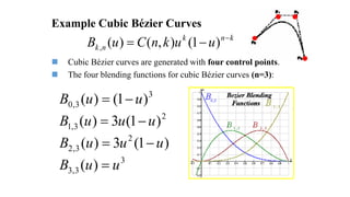
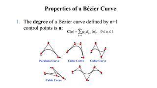
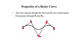
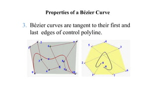
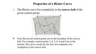
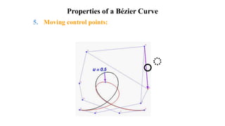
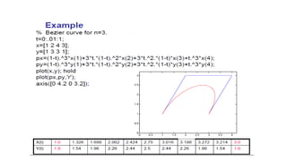
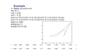
1. Welcome
TO
Our
Presentation

2. Introducing my group members
Md. Ilias Bappi
ID: 131-15-2266
Ferdous Ahamad
ID:131-15-2408
Md.Kawsar Hamid
ID:131-15-2223
Md. Jahirul Shahed
ID: 131-15-2479
Saiful Islam
ID:131-15-2516

3. Our Presentation
Topic
Bézier
curve

4. Hermite curve
The hermite curve is the curve for the data P,Q, v, and w. the four
polynomials in figure are called the hermite functions, or hermite
basis functions.
Here,
P and Q are points, and velocity vectors
v and w
Figure: The four Hermite polynomials.

5. Matrix formulation of Hermite curve
The first factor is the geometry matrix (G)
The middle matrix, called the basis matrix (M)
Thus, in brief, the Hermite curve can be written
γ(t) = GMT(t).
This basis matrix M that lists the coefficients of some polynomials, and the vector T(t).

6. Bézier curve
• Bézier curve defined by four points P1, . . . , P4.
• The curve starts at P1, finishes at P4, and has initial velocity 3(P2
−P1) and final velocity 3(P4 −P3), as shown in Figure.

7. Finding a point on a Bézier Curve
• A simple way to find the point C(u) on the curve
for a particular u is
1.To plug u into every basis function
2.Compute the product of each basis function and its
corresponding control point
3.Add them together.
10),()( ,
0
 
uuBu nk
n
k
kpC
),,( kykk zyxp nk 0
knk
nk uuknCuB 
 )1(),()(,

9. Derivatives or Design
Techniques Using
Bézier Curve

12. Design Techniques Using Bézier Curve
(Weights)
Multiple control points at a single coordinate position
gives more weight to that position.

13. Design Techniques Using Bézier Curve
(Closed Curves)
Closed Bézier curves are generated by specifying
the first and the last control points at the same
position.
Note: Bézier curves are polynomials which cannot represent
circles and ellipses.
0
1
2
3
4
5
6
7
8

14. Example Cubic Bézier Curves
knk
nk uuknCuB 
 )1(),()(,
 Cubic Bézier curves are generated with four control points.
 The four blending functions for cubic Bézier curves (n=3):
3
3,3
2
3,2
2
3,1
3
3,0
)(
)1(3)(
)1(3)(
)1()(
uuB
uuuB
uuuB
uuB




3,1
B

15. Properties
of
Bézier Curves

16. Properties of a Bézier Curve
10),()( ,
0
 
uuBu nk
n
k
kpC
1. The degree of a Bézier curve defined by n+1
control points is n:
Parabola Curve Cubic Curve Cubic Curve
Cubic Curve

17. Properties of a Bézier Curve
2. The curve passes though the first and the last control point
C(u) passes through P0 and Pn.

18. Properties of a Bézier Curve
3. Bézier curves are tangent to their first and
last edges of control polyline.
1
2
0
3
4
5
8
7
6
10
9
0
1
2
3
4
5
6
7
8

19. Properties of a Bézier Curve
4. The Bézier curve lies completely in the convex hull of the
given control points.
 Note that not all control points are on the boundary of the convex
hull. For example, control points 3, 4, 5, 6, 8 and 9 are in the
interior. The curve, except for the first two endpoints, lies
completely in the convex hull.

20. Properties of a Bézier Curve
5. Moving control points:

23. Thank You