Download as PDF, PPTX


![M R V
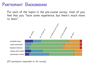
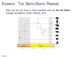
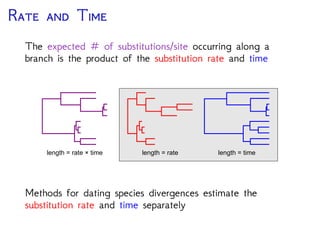
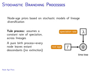
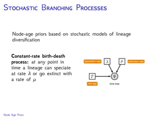
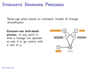
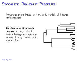
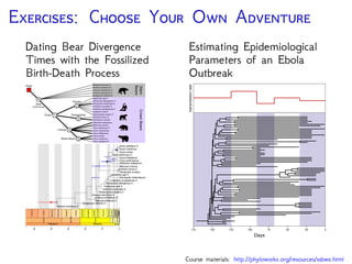
Are our models appropriate across all data sets?
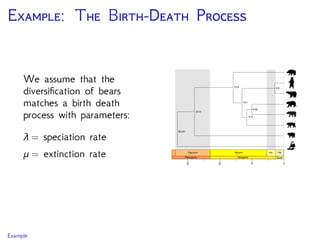
cave bear
American
black bear
sloth bear
Asian
black bear
brown bear
polar bear
American giant
short-faced bear
giant panda
sun bear
harbor seal
spectacled
bear
4.08
5.39
5.66
12.86
2.75
5.05
19.09
35.7
0.88
4.58
[3.11–5.27]
[4.26–7.34]
[9.77–16.58]
[3.9–6.48]
[0.66–1.17]
[4.2–6.86]
[2.1–3.57]
[14.38–24.79]
[3.51–5.89]
14.32
[9.77–16.58]
95% CI
mean age (Ma)
t2
t3
t4
t6
t7
t5
t8
t9
t10
tx
node
MP•MLu•MLp•Bayesian
100•100•100•1.00
100•100•100•1.00
85•93•93•1.00
76•94•97•1.00
99•97•94•1.00
100•100•100•1.00
100•100•100•1.00
100•100•100•1.00
t1
Eocene Oligocene Miocene Plio Plei Hol
34 5.3 1.823.8 0.01
Epochs
Ma
Global expansion of C4 biomass
Major temperature drop and increasing seasonality
Faunal turnover
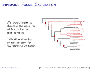
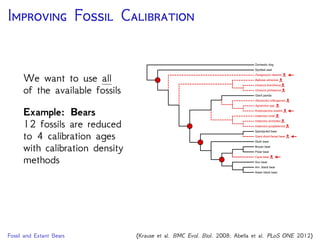
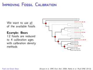
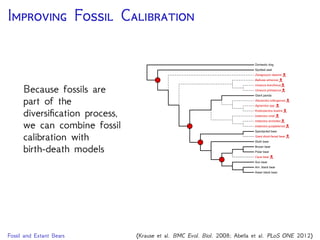
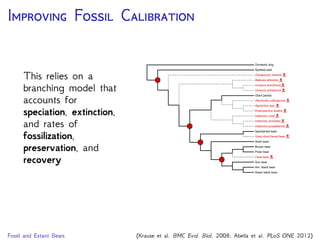
Krause et al., 2008. Mitochondrial genomes reveal an
explosive radiation of extinct and extant bears near the
Miocene-Pliocene boundary. BMC Evol. Biol. 8.
Taxa
1
5
10
50
100
500
1000
5000
10000
20000
0100200300
MYA
Ophidiiformes
Percomorpha
Beryciformes
Lampriformes
Zeiforms
Polymixiiformes
Percopsif. + Gadiif.
Aulopiformes
Myctophiformes
Argentiniformes
Stomiiformes
Osmeriformes
Galaxiiformes
Salmoniformes
Esociformes
Characiformes
Siluriformes
Gymnotiformes
Cypriniformes
Gonorynchiformes
Denticipidae
Clupeomorpha
Osteoglossomorpha
Elopomorpha
Holostei
Chondrostei
Polypteriformes
Clade r ε ΔAIC
1. 0.041 0.0017 25.3
2. 0.081 * 25.5
3. 0.067 0.37 45.1
4. 0 * 3.1
Bg. 0.011 0.0011
OstariophysiAcanthomorpha
Teleostei
Santini et al., 2009. Did genome duplication drive the origin
of teleosts? A comparative study of diversification in
ray-finned fishes. BMC Evol. Biol. 9.](https://image.slidesharecdn.com/bayesiandivtimessb-150520094854-lva1-app6892/85/Bayesian-Divergence-Time-Estimation-70-320.jpg)
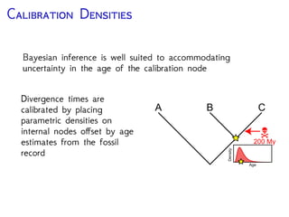
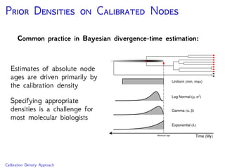
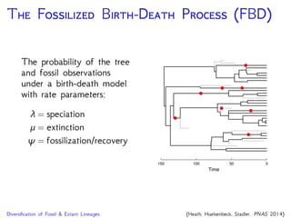
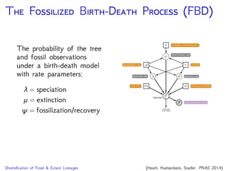
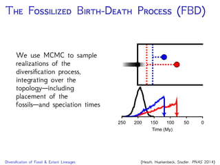
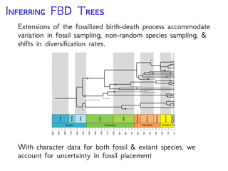
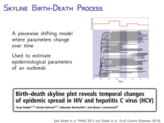

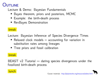

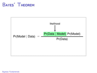
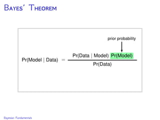
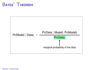
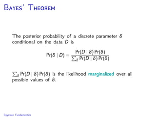
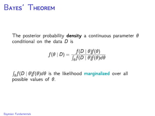
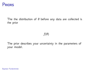
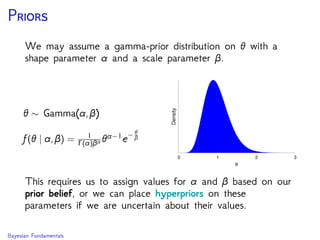
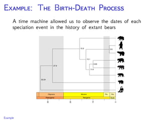
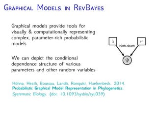
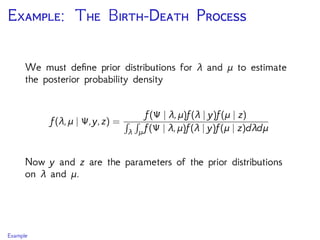
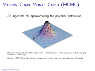
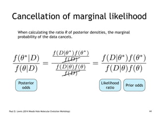
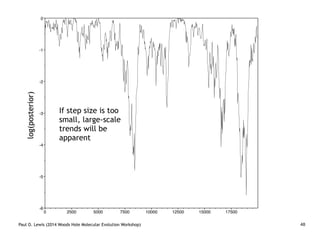
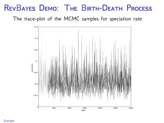
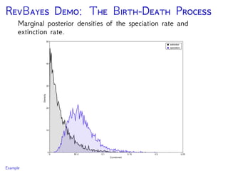
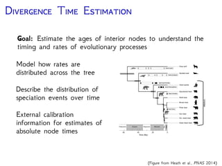
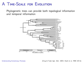
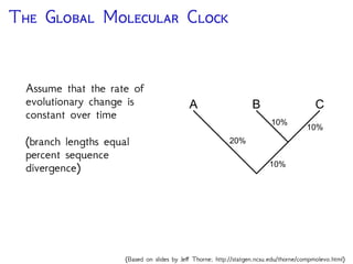
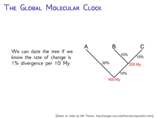
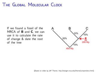
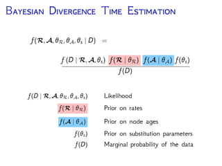
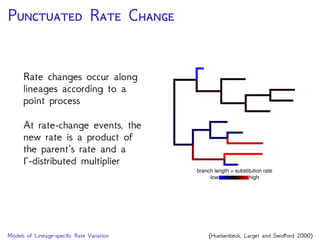
The document discusses Bayesian divergence time estimation in phylogenetics, focusing on Bayesian fundamentals, including Bayes' theorem, priors, and the birth-death process. It highlights the importance of relaxed clock models and MCMC methods for inferring species divergence times. Various tools, including RevBayes and graphical models, are introduced for visual representation and computational analysis of complex probabilistic models.