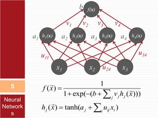
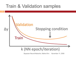
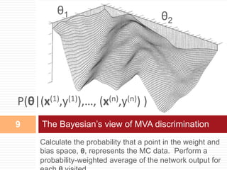
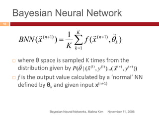
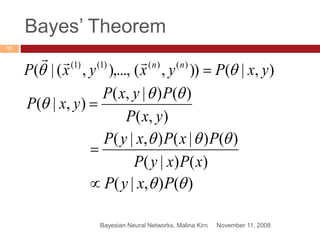
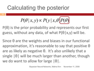
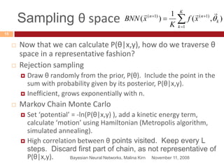
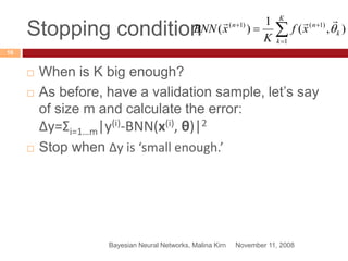
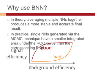
Bayesian Neural Networks

BAYESIAN NEURAL
NETWORKS
Introduction
Neural networks
Bayesian neural networks
Malina Kirn, Scientific ComputingNovember 11,
2008
1

Approximating the probability
November 11, 2008Bayesian Neural Networks, Malina Kirn
2
 We wish to develop some algorithm that will
approximate the probability that a given event is
signal.
 The MC then has the input distribution (x(1)…x(n))
and the truth/target value (y(1)…y(n)), which will
take the value of 0 (for background) or 1 (for
signal).
 We want P(y(n+1)=1|x(n+1),(x(1),y(1))…(x(n),y(n)))
 An intelligent algorithm will capitalize on
correlations (possibly non-linear) in x.

Measure the frequency of MC signal and background
events in a particular bin in physical space and assign
the probability of a real event as signal accordingly.
The Frequentist’s view of MVA discrimination3
P(y(n+1)=1|x(n+1),(x(1),y(1))…(x(n),y(n)))
x1
x2

NN: Approximate the shape of the physical space
with a sum of weighted and shifted non-linear
functions. Iterate to find the appropriate parameters
The Computationalist’s view of MVA
discrimination
4
Δy=Σi=1…n|y(i)-f(x(i), θ)|2
θ1
θ2

Neural
network
s
5
f(x)
h1(x) h2(x) h3(x) h4(x)
x1 x2 x3
v1 v2 v3 v4
u11
u34
u24
b
a1 a2 a3 a4
)tanh()(
)))((exp(1
1
)(





i iijjj
j jj
xuaxh
xhvb
xf



Neural
Network
s

November 11, 2008Bayesian Neural Networks, Malina Kirn6
Steepest Descent
 Labeling all network parameters uij, vj, (weights)
aj, and b (biases) as θ, then the goal is to iterate
through θ space minimizing the error.
 Typically done via Steepest Descent (SD), though
there are many alternatives.
 θ(k+1)=θ(k)-c (Δy(θ(k)))
 When to stop evolving?
Δ

Train & Validation samples
7
Δy
k (NN epoch/iteration)
Stopping condition
Validation
Train

Number of hidden nodes and
layers?
8
 A NN with an infinite number of hidden nodes
can approximate an arbitrarily complicated
function.
 Too many hidden nodes/layers and you
introduce instability.
 Common to characterize a network topology
as good based on how well it performs on the
validation sample.
 Do this too often and you can no longer
estimate the error of the NN from the validation
sample. Use a third sample, called the test
sample, to do so.

Calculate the probability that a point in the weight and
bias space, θ, represents the MC data. Perform a
probability-weighted average of the network output for
The Bayesian’s view of MVA discrimination9
P(θ|(x(1),y(1)),…, (x(n),y(n)) )
θ1 θ2

Bayesian Neural Network
10



K
k
k
nn
xf
K
xBNN
1
)1()1(
),(
1
)( 

 where θ space is sampled K times from the
distribution given by
 f is the output value calculated by a ‘normal’ NN
defined by θk and given input x(n+1)
)),)...(,(|( )()()1()1( nn
yxyxP



Bayes’ Theorem
11
)()|(
)()|(),|(
xPxyP
PxPxyP 

),|()),(),...,,(|( )()()1()1(
yxPyxyxP nn
 

),(
)()|,(
),|(
yxP
PyxP
yxP

 
)(),|(  PxyP

Calculating the posterior
12
)(),|(),|(  PxyPyxP 


n
i
ii
xyPxyP 1
)()(
),|(),|( 
This is exactly what the NN is doing! f(x(i),θ) is the
probability that y(i)=1 given x(i) and θ and 1-f(x(i),θ)
is the probability that y(i)=0.
)()(
1)(
1
)(
)),(1(),(),|(
ii
yin
i
yi
xfxfxyP 

  


Calculating the posterior
13
)(),|(),|(  PxyPyxP 
P(θ) is the prior probability and represents our first
guess, without any data, of what P(θ|x,y) will be.
Since θ are the weights and biases in our functional
approximation, it’s reasonable to say that positive θ
are as likely as negative θ. It’s also unlikely that a
single |θ| will be much larger than another, though
we do want to allow for large |θ|.

Priors & hyperpriors
14
 Model the prior probability for each θ as a gaussian
centered about zero with width σ.
 Typically have classes - u’s, v’s (weights), a’s, b (biases)
and one σ for each class (σu, σv, σa, σb)
 What should σ be? Model P(σ), the hyperprior, as a
function that allows large values with a few chosen
parameters, the hyperparameters.
 





 
 

 dP
x
dPPP )(
2
exp
2
1
)()|()( 2
2

Sampling θ space
15
 Now that we can calculate P(θ|x,y), how do we traverse θ
space in a representative fashion?
 Rejection sampling
 Draw θ randomly from the prior, P(θ). Include the point in the
sum with probability given by its posterior, P(θ|x,y).
 Inefficient, grows exponentially with n.
 Markov Chain Monte Carlo
 Set ‘potential’ = -ln(P(θ|x,y) ), add a kinetic energy term,
calculate ‘motion’ using Hamiltonian (Metropolis algorithm,
simulated annealing).
 High correlation between θ points visited. Keep every L
steps. Discard first part of chain, as not representative of
P(θ|x,y).



K
k
k
nn
xf
K
xBNN
1
)1()1(
),(
1
)( 


Stopping condition
16
 When is K big enough?
 As before, have a validation sample, let’s say
of size m and calculate the error:
Δy=Σi=1…m|y(i)-BNN(x(i), θ)|2
 Stop when Δy is ‘small enough.’



K
k
k
nn
xf
K
xBNN
1
)1()1(
),(
1
)( 


Why use BNN?
17
 In theory, averaging multiple NNs together
produces a more stable and accurate final
result.
 In practice, single NNs generated via the
MCMC technique have a smaller integrated
area under the ROC curve than the
corresponding BNN.
background efficiency
signal
efficiency
good
bad

Bayesian Neural Networks

More Related Content

What's hot

Similar to Bayesian Neural Networks

Recently uploaded

Bayesian Neural Networks