This thesis analyzes neural coding in the hippocampus using statistical modeling techniques. It summarizes experiments recording neural activity from place cells in rats navigating a T-maze. Generalized linear models are used to model each neuron's firing rate based on position and firing history. Goodness of fit tests show many neurons are well modeled. An algorithm is derived to decode position from the ensemble activity using Bayes' rule and numerical integration of the exact posterior distribution. The models and decoding algorithm are applied to analyze the hippocampal population code.

1. A Principled Statistical Analysis
of Discrete Context-Dependent
Neural Coding
Yifei Huang
Thesis Advisor: Prof. Uri Eden
April 14th, 2010
1

2. Overview
• Basics of Neural Representations
• Point Process Modeling of Neural Systems
• Hippocampal Data Analyses
– Encoding
– Decoding
– Hypothesis Tests
– Other Topics
• Summary
2

3. Spikes are the Language of Neurons
Electrical Recordings
• Neurons send information in the form of an Electrical Impulse
electrical impulse that is termed a “spike”.
Electrode
Spike Train
Spike
A Neuron
Slide Courtesy of Mike Prerau 3

4. Place cells in Hippocampus
Human:
Rat:
y position (m)
Firing
activity of
a single
place cell:
4
x position (m)

5. Neural Coding
Input: Output:
Neural
X: Spiking N:
System
Example of x and N – hippocampal system
Challenge: construct a probability model of the relationship
between the spike sequence and biological or behavioral
variables x
Point Process Model: p( N | x)
5

6. The Decoding Problem
Neuron 1
p(x|N1,…,NC) Parameters
Biological
?
Stimulus
Neuron 2
Parameters
…
Neuron C
Parameters
Challenge: track the biological stimulus/behavior signal
as it evolves. e.g. Position 6

7. Conditional Intensity Function (CIF) and
the Likelihood Function
• Point Processes are modeled with CIF
Pr(Spike in (t , t + ∆t ) | H t )
λ (t | H t ) = lim = g(t, x(t), Ht; θ)
∆t → 0 ∆t
• In discrete time the log-likelihood for observing a
spike train is:
K K
log L = ∑ log[λ (tk | N1:k )∆t ]∆N k − ∑ λ (tk | N1:k )∆t
k =1 k =1
t1 t2 t3 t4 t5 t6 t7
ΔN1 ΔN2 ΔN3 ΔN4 ΔN5 ΔN6 ΔN7
0 0 1 0 0 0 1
7

8. Experimental Paradigm and Data
Decision Point
A rat was trained to
alternate between left /
right turns on a T-maze.
- Recordings were made from
47 hippocampal place cells.
- Position data were recorded Left-turn trial Right-turn trial
at 30 Hz (frames/sec).
Data acquisition by M.P. Brandon and A.L. Griffin from Prof. Hasselmo’s lab
Challenge: p(Ν | x, context), p(x|N1,…,NC), prediction of the
future turn direction
8

9. Encoding Recorded firing
activity of an
Analysis individual neuron
9

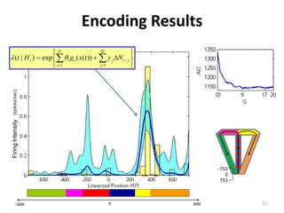
10. Generalized Linear Models
• Assume that the firing activity in each neuron follows a
point process with CIF:
Spline Basis
Functions
P Q

λ (t | H t ) = exp∑ θ i g i ( x(t )) + ∑ γ j ∆N t − j 
 i =1 j =1 
History Dependent
λ(t) Component
x(t)
• Compute the ML estimates for [θ1,…,θP, γ1,..., γQ]
10

11. Encoding Results
P Q

λ (t | H t ) = exp∑ θ i g i ( x(t )) + ∑ γ j ∆N t − j 
 i =1 j =1 
Firing Intensity
-753
0
753
x(t)
-800 0 800 11

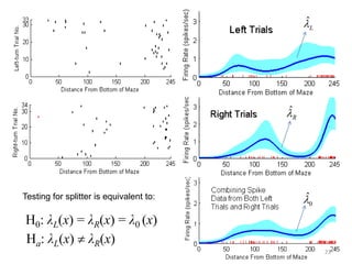
12. Goodness-of-fit Results
P Q

Time-rescaling Theorem λ (t | H t ) = exp∑ θ i g i ( x(t )) + ∑ γ j ∆N t − j 
(Meyer,1969 ; Papangelou,1972)  i =1 j =1 
λ (t | H t )dt
si +1
zi = ∫
si
~ i.i.d. exp(1)
KS Plot KS Plot
ui = 1 − exp(− zi )
~ i.i.d. Uniform [0,1]
Kolmogorov-Smirnov
Statistic
(Chakravarti et al., 1967)
KS = max Femp − F
F(u) = u Q=0 Q = 17
12

13. Ensemble results
• For an ensemble of 47 neurons:
– All neurons displayed highly specific position-
dependent firing
– Frequent peaks at multiple locations along the
maze
– 19 well fit by the inhomogeneous Poisson model
as measured by the KS test
– 29 well fit by the history-dependent point process
model
– Structure shown in the ACF reduced when a
simple history component was added
13

14. From Encoding to Decoding
( ) 1 ∆N k
1
At the kth time step, Pr(∆N | xk ) ∝ exp(−λ ) ⋅ λ
1
k
1
k k
Neuron 1
Parameters
? Pr(∆N k2 | xk )
p ( xk | ∆N k , , ∆N kC )
1
Neuron 2
Parameters
… Pr(∆N kC | xk )
Neuron C
Parameters
14

15. Derivation of the Decoding Algorithm
• Bayes Rule
C
p ( xk | ∆N ,  , ∆N ) ∝ ∏ Pr(∆N kc | xk ) p ( xk )
1
k
C
k
c =1
ρk
• Chapman-Kolmogorov equation
p( xk ) = ∫ p( xk | xk −1 ) p ( xk −1 | ∆N k −1 ,  ∆N kC−1 )dxk −1
1
ρk-1
• Numerical integration of exact posterior distribution
C
ρ k ∝ ∏ Pr(∆N kc | xk ) ∫ p( xk | xk −1 ) ρ k −1dxk −1
c −1
15

16. Decoding Analysis
Point Process Filter Derivation:
•State Model - State transition probability: p ( xk | xk −1 )
p (d k ) ~ N (0, σ 2 )
f(xk-1)
dk := xk = xk-1 + dk if the animal does not
xk – xk-1 move through the connection point
Alternatively – empirical state model
p (d k ) ~ N ( f ( xk −1 ), σ 2 )
f(xk-1) is the expected movement of
xk-1 the animal based on training data
•Conditional Intensity Models – Spline-based GLMs
•Decode algorithm - Numerical integration of exact posterior distribution
C
ρ k ∝ ∏ Pr(∆N kc | xk ) ∫ p ( xk | xk −1 ) ρ k −1dxk −1
c −1
16

17. Posterior Density
0.02
Posterior Density (ρk )
Linearized Position
-753
0
753
0 800 17
-800

18. 2-D Decoding Movie
Actual Position
Predicted Position
95% CI
18

19. Decoding
Results
•2D Mean Squared
Error:
(5.71 cm)2
•Coverage
Probability:
83.10 %
•Fraction of turn
decisions correctly
estimated:
66/69
19

20. Hypothesis Tests for Differential Firing
Motivation: which neurons fire differently under
two discrete contexts (left vs. right trial)?
Recorded Data for an Spiking activity before different turns:
Individual Neuron
20

21. Tests for Differential Firing
• Classic approach:
1. Break stem into 4-7
equally sized spatial
bins.
2. Perform 2-way ANOVA
on space and context
3. Look for significance in
context or interaction
terms.
21

22. Tests for Differential Firing
• ANOVA issues:
– Doesn’t capture spiking structure
– Asymptotic requirements are often not met
– Stationarity assumption
– Highly sensitive to number of bins
– Surprising previous decoding analysis
• Alternate approach:
– Tests based on point process models with
established goodness-of-fit procedures
22

23. λL
ˆ
λR
ˆ
Testing for splitter is equivalent to: λ0
ˆ
H0: λL(x) = λR(x) = λ0 (x)
Ha: λL(x) ≠ λR(x)
23

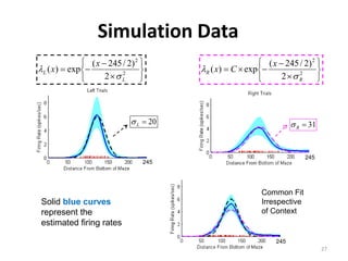
24. Test Statistics for Differential Firing
• Integrated squared error statistic:
ISE = ∫
0
D
(ˆ
 L

ˆ
0 ) ( ˆ
R
ˆ
0 )
 λ ( x) − λ ( x) 2 + λ ( x) − λ ( x) 2  dx


• Maximum difference statistic:
MD = max λL ( x) − λR ( x)
ˆ ˆ
x∈[ 0 , D ]
• Likelihood ratio statistic:
L0
W = −2 log
L1
24

25. Computing Sampling Distributions
• Nonparametric Bootstrap:
– Permute/sample from trial labels to
construct surrogates for each context.
• Parametric Bootstrap:
– Generate spikes according to λ0 ( x ) for
ˆ
each context.
– Alternative: sample λ0i ( x ) based on
ˆ
estimated model covariance, then generate
spikes.
25

26. Asymptotic distribution of W
– The asymptotic distribution of the LR Test Statistic:
L0
W = −2 log ~ χp
2
L1
p - number of constrained parameters under H0
– Asymptotic result holds when data size goes to
infinity; simulation study shows fast convergence
26

27. Simulation Data
 ( x − 245 / 2) 2   ( x − 245 / 2) 2 
λL ( x) = exp−  λR ( x) = C × exp− 
 2 ×σ L
2
  2 ×σ R
2

σ L = 20 σ R = 31
245
245
Common Fit
Solid blue curves Irrespective
represent the of Context
estimated firing rates
245
27

28. Test Results for Simulated Data
σ L = 20 σ R = 31 σ R = 34
Test p-value p-value
ANOVA Main effect: 0.865 Main effect: 0.706
(4 bins) Interaction effect: 0.202 Interaction effect: 0.728
ANOVA Main effect: 0.995 Main effect: 0.729
Interaction effect: 0.225 Interaction effect: 0.001
(6 bins)
0.003
ISE 0.021
0.001
MD 0.030
<0.001
LR (Asymp. χ2) 0.002 28

29. λ1
ˆ Back to the Real
Data Example…
Empirical and Asymptotic
Distributions of the LR Test Stat
L0
λ
ˆ
2
W = −2 log ~ χ p
2
L1
Blue Curve: χ24
Yellow Bars:
Bootstrap samples
λ0
ˆ
29

30. Real Data Results
Test p-value Recorded Data
for an Individual
Main effect: 0.872 Neuron
ANOVA
(4 bins) Interaction effect: 0.461
Main effect: 0.790
ANOVA
(6 bins) Interaction effect: 0.843
ISE <0.001
MD <0.001
LR (Asymp. χ2) <0.001
30

31. Summary of Test Results
• From simulation study
– Tests based on point process models tend to be
more powerful and robust compared to ANOVA
• From real data analysis
– The three proposed tests can capture differential
firing based on the fine structure of data
– Simple point process models were able to detect
differential firing in a population for which no
splitting behavior was previously identified
31

32. Other Topics
Relationships between spikes and neural oscillation
Theta Rhythmicity &Theta Precession
x(t)
720
ϕ(t)
Point Process Models:
λ (t H t ) = g (t , x(t ),φ (t ), H t ;θ )
180 32

33. Conclusions
• Theory/Methods developed
– Model identification paradigm for firing activity of
hippocampal neurons
– Exact decoding on general topologies
– Hypothesis test framework
• Understanding of the brain
– Decoding results suggest the neuron ensemble from
hippocampus contain information for future turn
direction
– Theta rhythmicity is an essential component for
hippocampal neural firing
33

34. Acknowledgements
Advisor: Uri Eden
Experimental Data:
Mark Brandon
Amy Griffin
Professor Michael Hasselmo
Lab Members:
Michael Prerau Eugene Zaydens
Liang Meng Kyle Lepage
Committee Members:
Ashis Gangopadhyay Michael Hasselmo
Dan Weiner Kostas Kardaras
34