This document discusses quantitative electromyography (QEMG) and what can be assessed using EMG. It outlines various muscle fiber characteristics and motor unit organization that EMG can evaluate, including number of fibers, grouping, and transmission at the neuromuscular junction. Parameters that can be quantified from concentric and monopolar EMG signals are described, such as spontaneous activity, motor unit potential (MUP) shape, recruitment, and dynamic changes over time. Various MUP parameters that provide information on motor unit size and characteristics are also defined. The document compares these parameters in evaluating different muscle disorders like neuropathy, myopathy and provides examples of quantitative analyses.

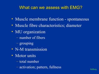
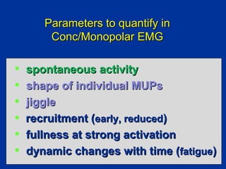
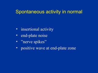
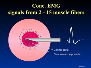
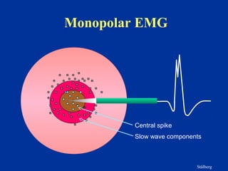
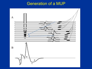
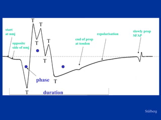
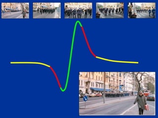
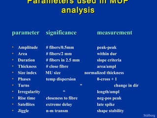
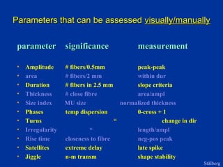
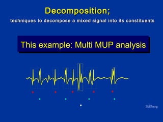
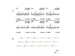
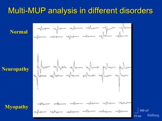
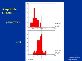
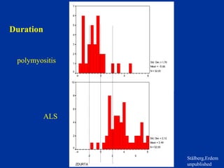
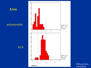
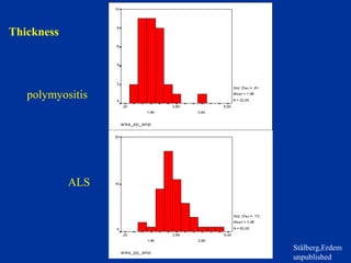
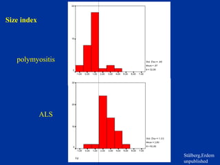
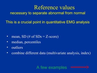
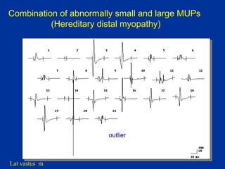
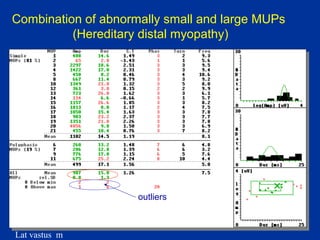
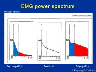
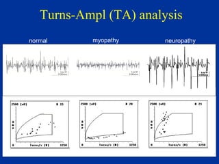
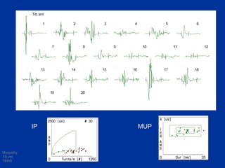
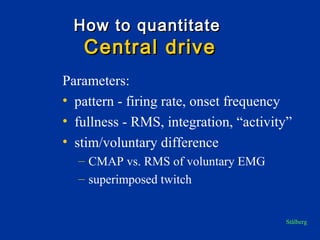
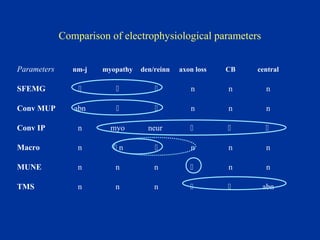
1. Erik Stålberg
Uppsala
Sweden

2. What can we assess with EMG?What can we assess with EMG?
• Muscle membrane function - spontaneous
• Muscle fibre characteristics; diameter
• MU organization
– number of fibers
– grouping
• N-M transmission
• Motor units
– total number
– activation; pattern, fullness Stålberg

3. Parameters to quantify inParameters to quantify in
Conc/Monopolar EMGConc/Monopolar EMG
• spontaneous activityspontaneous activity
• shape of individual MUPsshape of individual MUPs
• jigglejiggle
• recruitment (recruitment (early, reducedearly, reduced))
• fullness at strong activationfullness at strong activation
• dynamic changes with time (dynamic changes with time (fatiguefatigue))

5. Spontaneous activity in normal
• insertional activity
• end-plate noise
• ”nerve spikes”
• positive wave at end-plate zone

7. Conc. EMG
signals from 2 - 15 muscle fibers
Stålberg
Central spike
Slow wave components

8. Monopolar EMG
Stålberg
Central spike
Slow wave components

9. Generation of a MUP

11. opposite
side of nmj
end of prop
at tendon
slowly prop
SFAPrepolarisation
T
T
T
T
duration
start
at nmj
phase
Stålberg
T
T
T

12. 27

13. Parameters used in MUPParameters used in MUP
analysisanalysis
parameterparameter significancesignificance measurementmeasurement
• Amplitude # fibers/0.5mm peak-peak
• Area # fibers/2 mm within dur
• Duration # fibers in 2.5 mm slope criteria
• Thickness # close fibre area/ampl
• Size index MU size normalized thickness
• Phases temp dispersion 0-cross + 1
• Turns “ change in dir
• Irregularity “ length/ampl
• Rise time closeness to fibre neg-pos peak
• Satellites extreme delay late spike
• Jiggle n-m transm shape stability
Stålberg

14. Parameters that can be assessedParameters that can be assessed visually/manuallyvisually/manually
parameterparameter significancesignificance measurementmeasurement
• Amplitude # fibers/0.5mm peak-peak
• area # fibers/2 mm within dur
• Duration # fibers in 2.5 mm slope criteria
• Thickness # close fibre area/ampl
• Size index MU size normalized thickness
• Phases temp dispersion 0-cross + 1
• Turns “ change in dir
• Irregularity “ length/ampl
• Rise time closeness to fibre neg-pos peak
• Satellites extreme delay late spike
• Jiggle n-m transm shape stability
Stålberg

16. This example: Multi MUP analysis
techniques to decompose a mixed signal into its constituentstechniques to decompose a mixed signal into its constituents
Decomposition;Decomposition;
Stålberg

17. A
B
C

18. 500 uV
10 ms
NormalNormal
NeuropathyNeuropathy
MyopathyMyopathy
Multi-MUP analysis in different disordersMulti-MUP analysis in different disorders
Stålberg

19. A
m
p
L
I
t
u
d
e

20. Amplitude
Measured peak-peak
* note that jiggle will reduce
mean amplitude
(measured
after averaging)

21. Duration

22. Parameters for duration-Parameters for duration-
measurementmeasurement
Stålberg

23. area

24. Area
Positive and negative signal
segment between duration
cursors; mVmsec

25. Thick-
ness

26. Thickness
Calculated as
area/ampl
(In a triangle, area/height=base/2)

27. Size
index
Sonoo,Stålberg 1993

28. Size index
An algorithm to normalize
“thickness” for amplitude
SI=2 log(ampl) + area/ampl

29. C X
E
L
P
M
O
T
I Y
Phases, turns

30. Phases, turns
Way to express complexity
>4 phases = polyphasic
> 5 turns = complex, serrated

31. I R
R
L
U
G
E
T
I
R
A Y

32. The jiggle

33. The jiggle

34. The jiggle

35. The jiggle

36. The jiggle

37. Jiggle in normal and abnormalJiggle in normal and abnormal
MUPsMUPs
Stålberg
Normal
ALS

38. So, shall I use all these
parameters??
Which one is best?
Let us look at the diagnostic power of
a few parameters

39. Amplitude
(Tib.ant.)
ZAMPTA
8
6
4
2
0
-2
-4
10
8
6
4
2
0
Std. Dev = 1,11
Mean = -1
N = 32,00
ZAMPTA
8
6
4
2
0
-2
-4
12
10
8
6
4
2
0
Std. Dev = 1,21
Mean = 1
N = 52,00
0.87
,13
polymyositis
ALS
Stålberg,Erdem
unpublished
SD
SD
-2SD +2SD

40. Duration
ZDURTA
8
6
4
2
0
-2
-4
7
6
5
4
3
2
1
0
Std. Dev = 1,76
Mean = -1
N = 32,00
ZDURTA
8
6
4
2
0
-2
-4
10
8
6
4
2
0
Std. Dev = 2,12
Mean = 3
N = 52,00
0.88
.46
polymyositis
ALS
Stålberg,Erdem
unpublished

41. Area
ZAREATA
8
6
4
2
0
-2
-4
10
8
6
4
2
0
Std. Dev = 1,14
Mean = -1
N = 32,00
ZAREATA
8
6
4
2
0
-2
-4
12
10
8
6
4
2
0
Std. Dev = 1,10
Mean = 1
N = 52,00
.36
0,85
polymyositis
ALS
Stålberg,Erdem
unpublished

42. Thickness
polymyositis
ALS
Stålberg,Erdem
unpublished

43. Size index
polymyositis
ALS
Stålberg,Erdem
unpublished

44. No single parameter
Is superior to the other
In each case

45. Reference values
necessary to separate abnormal from normal
This is a crucial point in quantitative EMG analysis
• mean, SD (# of SDs = Z-score)
• median, percentiles
• outliers
• combine different data (multivariate analysis, index)
A few examples

46. Lat vastus m
outlier
Combination of abnormally small and large MUPs
(Hereditary distal myopathy)

47. Lat vastus m
Combination of abnormally small and large MUPs
(Hereditary distal myopathy)
outliers

48. InterferenceInterference
patternpattern

49. MethodsMethods
• recruitment analysis
• visual inspection (ampl, fullness)
• spectral analysis
• broad band filter analysis
• turns/amplitude analysis
• envelope, NSS, activity

50. Onset frequency
= freq of a MUP when recruited
Recruitment frequency
= freq. of 1st
MU when 2nd
is recruited
neuropathy ↑
myopathies ↓
Recruitment ratio (slight contraction)
= # discharges/# active MUs

51. Onset freq = 6 Hz
Recruitment freq = 9Hz
Recruitment ratio 20/4=5
Interference
6 8 10 12 14 16 18 20 Hz
normal
MU 1
MU 2
MU 3
MU 4
MU 5

52. Onset freq = 6 Hz
Recruitment freq = 9Hz
Recruitment ratio 20/4=5
Interference
6 8 10 12 14 16 18 20 Hz
normal
MU 1
MU 2
MU 3
MU 4
MU 5

53. Onset freq = 6 Hz
Recruitment freq = 9Hz
Recruitment ratio 20/4=5
Interference
6 8 10 12 14 16 18 20 Hz
normal
MU 1
MU 2
MU 3
MU 4
MU 5

54. 6 8 10 12 14 16 18 20 Hz
Onset= 6 Hz
Recruitment freq = 12
Recruitment ratio = 18/3=6
neurogenic
MU 1
(MU 2)
MU 3
MU 4

55. 6 8 10 12 14 16 18 20 Hz
Onset= 6 Hz
Recruitment freq = 7Hz
Recruit ratio = 10/3=3
myopathy
MU 1
MU 2
MU 3
MU 4

58. Stålberg, Daube 2003
Myopathy
Normal
Neuropathy

60. Frequency bands in EMG, schematic
0-50 200-300 1000 Hz
“LUCIA”
0-50 200-300 1000 Hz
0-50 200-300 1000 Hz

61. EMG power spectrumEMG power spectrum
Neuropathy Normal Myopathy
mBiceps brachii
A Fuglsang-Frederiksen

62. Turns-Ampl (TA) analysis
normal neuropathymyopathy

63. Myopathy
Tib ant
18446
IP MUP
Tib ant

64. How to quantitateHow to quantitate
Central driveCentral drive
Parameters:
• pattern - firing rate, onset frequency
• fullness - RMS, integration, “activity”
• stim/voluntary difference
– CMAP vs. RMS of voluntary EMG
– superimposed twitch
Stålberg

65. Comparison of electrophysiological parameters
Parameters nm-j myopathy den/reinn axon loss CB central
SFEMG    n n n
Conv MUP abn   n n n
Conv IP n myo neur   
Macro n  n  n n n
MUNE n n n  n n
TMS n n n   abn

66. Reasons for performing QEMG
• standardized way of measuring
• improved sensitivity
• results can be transferred
– from one time to the other - follow up
– from one physician to the other
– from on lab to the other
• reliable results also from less experienced
EMGers
• good during training