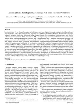
This document proposes an automated method for segmenting the fetal brain from 2D MRI slices that have been misaligned due to fetal motion. It combines fetal brain localization in each slice using Maximally Stable Extremal Regions (MSER) and Scale-Invariant Feature Transform (SIFT) features with a patch-based propagation and Conditional Random Field (CRF) to generate a segmentation mask for each slice. It then integrates this slice-by-slice segmentation with a motion correction process to iteratively refine the segmentation as the reconstruction proceeds. The method was tested on 66 datasets ranging from 22-39 weeks gestation and produced a motion corrected volume of diagnostic quality in 85% of cases while also generating a mean 93

1. Automated Fetal Brain Segmentation from 2D MRI Slices for Motion Correction
K. Keraudrena,∗
, M. Kuklisova-Murgasovab
, V. Kyriakopouloub
, C. Malamatenioub
, M.A. Rutherfordb
, B. Kainza
, J.V. Hajnalb
,
D. Rueckerta
aBiomedical Image Analysis Group, Department of Computing, Imperial College London, SW7 2AZ, UK
bCentre for the Developing Brain, Division of Imaging Sciences & Biomedical Engineering, King’s College London, St. Thomas’ Hospital, SE1 7EH, UK
Abstract
Motion correction is a key element for imaging the fetal brain in-utero using Magnetic Resonance Imaging (MRI). Maternal breath-
ing can introduce motion, but a larger effect is frequently due to fetal movement within the womb. Consequently, imaging is
frequently performed slice-by-slice using single shot techniques, which are then combined into volumetric images using slice-to-
volume reconstruction methods (SVR). For successful SVR, a key preprocessing step is to isolate fetal brain tissues from maternal
anatomy before correcting for the motion of the fetal head. This has hitherto been a manual or semi-automatic procedure. We
propose an automatic method to localize and segment the brain of the fetus when the image data is acquired as stacks of 2D slices
with anatomy misaligned due to fetal motion. We combine this segmentation process with a robust motion correction method,
enabling the segmentation to be refined as the reconstruction proceeds. The fetal brain localization process uses Maximally Sta-
ble Extremal Regions (MSER), which are classified using a Bag-of-Words model with Scale-Invariant Feature Transform (SIFT)
features. The segmentation process is a patch-based propagation of the MSER regions selected during detection, combined with a
Conditional Random Field (CRF). The gestational age (GA) is used to incorporate prior knowledge about the size and volume of
the fetal brain into the detection and segmentation process. The method was tested in a ten-fold cross-validation experiment on 66
datasets of healthy fetuses whose GA ranged from 22 to 39 weeks. In 85% of the tested cases, our proposed method produced a
motion corrected volume of a relevant quality for clinical diagnosis, thus removing the need for manually delineating the contours
of the brain before motion correction. Our method automatically generated as a side-product a segmentation of the reconstructed
fetal brain with a mean Dice score of 93%, which can be used for further processing.
Keywords:
Fetal MRI, Motion correction, Brain extraction, MSER, Bag-of-Words, SIFT
1. Introduction
Magnetic Resonance Imaging (MRI) is a primary tool for
clinical investigation of the brain and for neuroscience. High
resolution imaging with volumetric coverage using stacks of
slices or true three dimensional (3D) methods is widely avail-
able and provides rich data for image analysis. However such
detailed volumetric data generally takes several minutes to ac-
quire and requires the subject to remain still or move only small
distances during acquisition. Fetal brain imaging introduces a
number of additional challenges (Malamateniou et al., 2013).
Maternal breathing may move the fetus and the fetus itself can
and does spontaneously move during imaging. These move-
ments are unpredictable and may be large, particularly involv-
ing substantial head rotations. As a result, most fetal imag-
ing is performed using single shot methods to acquire two di-
mensional (2D) slices, such as single shot Fast Spin Echo, ss-
FSE, (Jiang et al., 2007) and Echo-Planar Imaging, EPI, (Chen
and Levine, 2001). These methods can freeze fetal motion, so
that each individual slice is generally artifact free, but stacks of
∗Corresponding author
Email address: kevin.keraudren10@imperial.ac.uk (K. Keraudren)
slices required to provide whole brain coverage may be mutu-
ally inconsistent.
Motion correction methods have revolutionized MRI of the
fetal brain by reconstructing a high-resolution 3D volume of
the fetal brain from such motion corrupted stacks of 2D slices.
Such reconstructions are valuable for both clinical and research
applications. They enable a qualitative assessment of abnormal-
ities suspected on antenatal ultrasound scans (Rutherford et al.,
2008) and are an essential tool to gain a better understanding of
the development of the fetal brain, pushing back the frontiers of
neuroscience (Studholme and Rousseau, 2013).
However, motion correction and reconstruction methods still
require a substantial amount of manual data pre-processing.
This makes direct clinical application of the methods imprac-
tical and is excessively time consuming in large cohort research
studies.
Therefore, we propose a fully automated tightly coupled seg-
mentation and reconstruction approach and present the follow-
ing contributions in this paper:
• We develop an automated method to mask the fetal brain
in every 2D slice of every 3D stack and designed it to serve
as a preprocessing step for motion correction (Section 3.2).
We thus seek an optimal segmentation that tackles both the
Preprint submitted to NeuroImage August 5, 2014

2. motion between different stacks as well as the motion be-
tween the interleaved packets of a single stack. This is
in contrast with a manual initialization of the motion cor-
rection procedure which typically propagates one manual
mask to the remaining stacks after rigid volumetric regis-
tration.
• We propose the application of a patch-based Random For-
est classifier to obtain a probabilistic slice-by-slice seg-
mentation of the brain, which is then refined with a 3D
Conditional Random Field (Section 3.2). The novelty of
this approach is to perform online learning with a global
classifier, whereas a typical patch-based segmentation uses
offline learning with a local classifier. We train our Ran-
dom Forest classifier using the partial segmentation result-
ing from the localization process described in Section 3.1.
• Given an approximate age of the fetus (gestational age),
we incorporate prior knowledge of the size and volume of
the fetal brain in both the detection (Section 3.1) and seg-
mentation processes (Section 3.2). In particular, we use an
estimation of the volume of the brain in order to improve
the probabilistic output of the Random Forest classifier.
• During motion correction, we take advantage of the align-
ment of all 2D slices to produce a 3D probabilistic seg-
mentation of the brain from all the slice-by-slice proba-
bilistic segmentations (Section 3.3). We use again a 3D
Conditional Random Field to update the segmentation of
the fetal brain, thus improving the reconstruction of a high-
resolution volume.
The outline of this paper is as follows. In Section 2, we
give an overview of related work for processing brain MRI. We
closely review in Section 3.1 our approach to localize the fetal
brain, first introduced in Keraudren et al. (2013), before show-
ing in Section 3.2 how to refine this localization from a bound-
ing box detection to a segmentation for all 2D slices of each
3D stack. In Section 3.3, we integrate this automated masking
with the motion correction procedure, evolving the mask of the
segmented brain during reconstruction. The resulting method
is then evaluated in two steps (Section 5), first assessing the
quality of the slice-by-slice segmentation, then comparing the
result of motion correction using a manual and an automated
initialization.
2. Related Work
2.1. Processing of conventional cranial MRI
Numerous methods have been proposed for an automated ex-
traction of the adult brain from MRI data, a problem also known
as skull stripping. The task is then to delineate the whole brain
in a motion free 3D volume. Most of the proposed methods
take advantage of the fact that the adult head is surrounded by
air and that the brain is thus the main structure in the image.
Brain extraction can then be performed using a region growing
process, such as in FSL’s Brain Extraction Tool (Smith, 2002)
and FreeSurfer’s Hybrid Watershed Algorithm (Segonne et al.,
2004), or using morphological operations and edge detection
such as in the Brain Surface Extractor of Shattuck et al. (2001).
A more general approach is to register the image to segment
with a brain template and use statistical models of brain tissues
(Warfield et al., 1998). Instead of a template, the new image can
also be registered to a set of already segmented images, called
an atlas (Van Leemput et al., 1999). Tissue classification can
then be performed, for instance by seeking similar patches from
the atlas in a local neighborhood and transferring their labels to
the new image, such as in BEaST (Eskildsen et al., 2012). Such
a patch-based segmentation has been applied to fetal data after
motion correction (Wright et al., 2012).
2.2. Brain localization in fetal MRI
Current methods to segment motion-free, high resolution
adult brain volumes cannot be straight-forwardly applied to the
extraction of the fetal brain from the unprocessed MR data. An-
quez et al. (2009) first proposed a method for extracting the
fetal brain from MRI with a low through-plane resolution, but
their proposed pipeline, which relies on detecting the eyes and
selecting a sagittal plane, is not robust to fetal motion. Taleb
et al. (2013) also proposed a method based on template match-
ing, but using templates from an age-dependent atlas of the fe-
tal brain. This method first defines a region of interest (ROI)
using the intersection of all scans and then registers this ROI
to an age dependent fetal brain template, before refining the
segmentation with a fusion step. Ison et al. (2012) and Kainz
et al. (2014) address the variability of fetal MRI through the use
of Machine Learning. Both methods rely on 3D features, ei-
ther 3D Haar-like features or dense rotation invariant features,
which are justified in cases of little motion, especially consider-
ing that the maternal anatomy is not moving and occupies most
of the image. In Keraudren et al. (2013), we proposed a method
to automatically select a bounding box around the fetal brain.
This method is robust to fetal motion as it first detects the fetal
brain in every 2D slice before aggregating the results in 3D. In
the present paper, we propose to leverage the result of the lo-
calization process to obtain a segmentation of the fetal brain in
the unprocessed data instead of a box detection.
2.3. Motion correction of the fetal head
Several methods have been proposed to correct fetal motion
and to reconstruct a single high-resolution 3D volume from or-
thogonal stacks of misaligned 2D slices. The most common
approach is slice-to-volume registration, where slices are itera-
tively registered to an estimation of the reconstructed 3D vol-
ume (Rousseau et al., 2006; Jiang et al., 2007; Gholipour et al.,
2010; Kuklisova-Murgasova et al., 2012). Another approach
proposed by Kim et al. (2010) formulates the motion correc-
tion problem as the optimization of the intersections of all slice
pairs from all orthogonally planned scans. A comprehensive
overview of these methods is given in Studholme and Rousseau
(2013).
In all proposed methods, the fetal head is considered a rigid
object moving independently from the surrounding maternal
tissues. Therefore, a manual initialization is required to iso-
late the fetal brain from the rest of the image. In both Rousseau
2

3. For every slice Detect MSER regions Filter by size
Classify into brain and non-brain
using SIFT features
Fit box with RANSAC
Figure 1: Pipeline to localize the fetal brain. Slice-by-slice, MSER regions are first detected and approximated by ellipses. They
are then filtered by size before being classified using histograms of 2D SIFT features. Finally, a 3D bounding box is fitted to the
selected MSER regions with a RANSAC procedure. In the last two steps, selected regions are shown in green while rejected regions
are shown in red.
et al. (2006) and Gholipour et al. (2010), a tight bounding box
is manually cropped for each stack of 2D slices. In Jiang et al.
(2007) and Kuklisova-Murgasova et al. (2012), the region con-
taining the fetal head is manually segmented in one stack, and
the segmentation is propagated to the other stacks after volume-
to-volume registration. Down-sampling the target volume fol-
lowed by up-sampling the mask can be performed to save time
during the manual segmentation. In Kim et al. (2010), a box
around the brain is manually cropped in one stack and propa-
gated to the other stacks after volume-to-volume registration.
An ellipsoidal mask, which evolves while the slices are aligned
is then used throughout the motion correction procedure.
Cropping only a box around the fetal brain is relatively fast
but may not be enough for the reconstruction to succeed, as tis-
sues outside the head of the fetus may mislead the registration.
However, manual segmentation requires time, about 10–20min
per stack of 2D slices, which can be a limitation for large scale
studies. Moreover, the assumption that a mask from one stack
can be propagated to all other stacks might not hold when the
fetus has moved a lot between the acquisitions of each stack.
Besides, slices are acquired one at a time and in an interleaved
manner in order to reduce the scan time while avoiding slice
cross-talk artifacts. In cases of extreme motion, the misalign-
ment between slices can cause a 3D mask to encompass too
much maternal tissue, thus requiring a slice-by-slice 2D seg-
mentation. In this paper, we propose to automatically segment
the fetal brain from the unprocessed data for the purpose of
motion correction. The main challenges are that the fetus is in
an unknown position, surrounded by maternal tissues, and may
have moved between the acquisitions of 2D slices.
3. Method
3.1. Bundled SIFT features brain localization pipeline
The pipeline for detecting the fetal brain from stacks of T2
weighted single shot images, outlined in Figure 1, is a slice-
by-slice approach combining state-of-the-art computer vision
methods. As the data is acquired as stacks of 2D slices mis-
aligned due to fetal motion, the brain is first detected indepen-
dently in every 2D slice before aggregating the results in 3D.
Besides the presence of motion, the main challenge is the large
variability of the appearance of the fetal brain in the 2D slices
due to the unknown orientation of the fetus as well as anatomi-
cal changes taking place during fetal development. In order to
address this challenge, the detection pipeline is based on a Bag-
of-Words model (Csurka et al., 2004), which is a classification
approach robust to large intra-class variability. SIFT features
(Scale-Invariant Feature Transform, Lowe, 1999) are used to
build a visual vocabulary, enabling the representation of image
regions as histograms of words. This is analogous with building
histograms of words to classify text documents. The rotation
invariance of SIFT features helps accommodate the unknown
orientation of the fetal brain, while their scale invariance atten-
uates the variations due to gestational age. In order to constrain
the search by incorporating prior knowledge about the expected
size of the fetal brain from the gestational age, SIFT features are
grouped within Maximally Stable Extremal Regions (MSER,
Matas et al., 2004), which can be filtered by size, resulting in
bundled SIFT features (Wu et al., 2009). The resulting Bag-of-
Words classifier is trained offline on training images manually
annotated with bounding boxes around the fetal brain.
MSER regions are characterized by homogeneous intensity
distributions and high intensity differences at their boundary.
They are connected components of the level sets of a grayscale
image whose boundaries are relatively stable over a small range
of intensity thresholds. They can be computed in quasi-linear
time by forming the component tree of the image (Najman et al.,
2004), a tree structure highlighting the inclusion relation of the
connected components of the level sets in the image. The po-
tential use of MSER regions to characterize the brain in MRI
was first proposed by Donoser and Bischof (2006) who used
volumetric MSER to segment simulated brain MR images. As
the brain and cerebrospinal fluid appear much brighter than the
surrounding bone and skin tissues in fetal T2 MRI, MSER re-
3

4. (a) (b)
Figure 2: (a) Detected brain (green box) and selected MSER
regions (red overlay). The top image shows a 2D slice while
the bottom image is an orthogonal cut through the stack of 2D
slices. (b) A Random Forest classifier is trained on patches
extracted in the selected MSER regions (green boxes selected
within the red overlay) and on patches extracted in a narrow
band at the boundary of the detected bounding box (red boxes
selected within the blue overlay).
gions are well suited to localize the brain. In order to define
the regions in which SIFT features will be computed, ellipses
are fitted to the MSER regions with a least-squares minimiza-
tion. As the brain is well approximated by an ellipsoid, this has
the advantage of recovering the shape of the brain even if the
detected MSER region only corresponds to a part of the brain.
Knowing the gestational age, those ellipses can be filtered by
size using estimates of the occipitofrontal diameter, OFD, and
the biparietal diameter, BPD, from 2D ultrasound studies (Sni-
jders and Nicolaides, 2003).
Following a typical Bag-of-Words model, SIFT features are
extracted from the training data and clustered using a k-means
algorithm to form a vocabulary from the cluster centers. Each
bundle of SIFT features can then be summarized as a histogram
of words by matching each SIFT feature to its nearest neighbor
in the vocabulary using the Euclidean distance. The classifica-
tion task is then performed using a linear kernel Support Vector
Machine (SVM) after normalization of the histograms with the
L2 norm. The SVM is trained using the bounding boxes man-
ually defined around the fetal brain. MSER regions of relevant
size that fit within these boxes are used as positive examples
whereas negative examples are taken further away from the fe-
tal head.
Finally, a RANdom SAmple Consensus procedure (RANSAC,
Fischler and Bolles, 1987) is used to find a best fitting cube
around the fetal head. The rationale for fitting a cube is that the
2D detection process performs best in the central slices of the
brain and that, due to the misalignment between slices, the de-
tected 2D ellipses might not define a proper 3D ellipsoid. The
dimensions of the 3D bounding cube are inferred from the ges-
tational age and purposefully over-estimate the size of the brain
by taking the 95th
centile of OFD to ensure that the full brain
will be processed during the segmentation step (Section 3.2).
As the detection process does not provide information on the
orientation of the brain, the selected box is simply aligned with
the image axes and is used to estimate the center of the brain in
the 3D volume. The RANSAC procedure proceeds as follows:
a restricted number of ellipses, typically 5, are randomly se-
lected and their centroid used to place a box. A score is then
computed by assessing the number of MSER regions fitting
within that box. This process is repeated, typically 1000 times,
and the box with the highest score is selected.
The result of the detection process is not only a bounding
box, but also a partial segmentation of the brain corresponding
to the selected MSER regions. Figure 2 shows an example of
the resulting mask. It can be noted that the selected MSER
regions do not cover the whole brain. In particular, due to the
size selection using BPD and OFD, the extremal slices of the
brain are unlikely to be included as they will be considered too
small. The brain extraction method proposed in Section 3.2 is
hence a propagation of this initial labeling within the region of
interest defined by the detected bounding box.
3.2. Brain extraction
By using a 2D slice-by-slice patch-based segmentation we
are able to propagate the initial labeling within the region of in-
terest obtained from the detection process described in Section
3.1. A typical patch-based segmentation searches each region
of the image to find the most similar patches within an atlas, a
training database with known ground truth segmentation. The
atlas is hence aligned with the image and a final segmentation
is obtained by fusing the votes from selected patches of atlas
images (Coup`e et al., 2010; Rousseau et al., 2011).
In our application, we seek to segment an image using a
sparse labeling of the same image. This sparse labeling cor-
responds to the periphery of the bounding box around the
brain (background label), as well as the selected MSER regions
(brain label), as shown in Figure 2. Therefore, we perform on-
line learning in contrast to conventional atlas based approaches,
which rely on offline training. Working on a single image at a
time excludes the need to normalize intensities or register the
volume to an atlas. Moreover, by learning from the same image,
we can adapt to the variability of the unprocessed fetal MR data.
In particular, we can work on 2D slices without prior knowledge
of the scan orientation relative to the fetal anatomy. Similarly to
Wang et al. (2013), we overcome the restriction of search win-
dows by using a single global classifier that compares patches
independently of their location in the image, instead of apply-
ing local classifiers. However, we chose a Random Forest clas-
sifier (Breiman, 2001), using 2D intensity patches as features,
to maintain a feasible training and testing speed. A k-nearest
neighbor classifier would have little training time, but its eval-
uation is a time-consuming process. The motivation for using
2D patches is that they are not corrupted by motion. Although
the 2D slices are not necessarily parallel in the anatomy of the
fetal brain, it can be expected that 2D patches small enough will
share sufficient similarities across different regions of the brain
to enable label propagation.
To obtain the initial sparse labeling on which the Random
Forest is trained, the mask obtained from Section 3.1 is first
4

5. preprocessed by drawing the ellipses fitted to the MSER re-
gions and filling any remaining hole. These regions provide
positive examples of 2D patches to learn the appearance of the
fetal brain, while negative examples are obtained by extract-
ing patches on a narrow band at the boundary of the detected
bounding box (Figure 2.b). The resulting classifier is then ap-
plied to the volume within the detected bounding box, to obtain
a probability map of brain tissues.
An estimation of the volume of the fetal brain from the gesta-
tional age (Chang et al., 2003) is used to refine the probabilistic
output of the Random Forest. This can be interpreted as a vol-
ume constraint in the segmentation process. For this purpose,
enough of the voxels most likely to be within the brain are se-
lected in the probability map to fill half of the estimated vol-
ume of the brain, and subsequently set to the highest probabil-
ity value. Likewise, enough of the voxels most likely to be part
of the background are selected to fill half of the background,
and set to the smallest probability value. The probability map
is then rescaled between [0, 1]. This corresponds to trimming
both sides of the intensity histogram of the probability map be-
fore rescaling it.
The probability map is then converted to a binary segmen-
tation using a Conditional Random Field (CRF, Lafferty et al.,
2001). This is a common approach in computer vision which
enables the combination of local classification priors (unary
term) with a global consistency constraint (pairwise term). We
use the formulation proposed by Boykov and Funka-Lea (2006)
which seeks to minimize the energy function:
E(l) =
p
D(p, lp) + λ
p,q
Vpq(lp, lq)
with the unary term (data cost) defined by the probabilistic pre-
diction of the Random Forest classifier:
D(p, lp) = − log(P(p|lp))
and a pairwise term (smoothness cost) penalizing labeling dis-
continuities between pixels of similar intensities:
Vpq(lp, lq) =
[lp lq]
p − q 2
e−(Ip−Iq)2
/2σ2
where p−q 2 is the distance between pixels taking image sam-
pling into account, |Ip −Iq| the intensity difference between pix-
els and σ an estimation of the image noise. λ is a weighting
between the data cost and the smoothness cost. High values of
λ will tend to assign the same label to large connected compo-
nents while small values of λ will tend to preserve the initial
labeling. This definition of the pairwise term is the same as the
edge weight of the graph cut used by Anquez et al. (2009) for
the segmentation of the fetal brain. An estimation of the image
noise is obtained by computing the difference between the im-
age and a Gaussian blurred version of the image. A more robust
method that would keep image edges from contributing to the
noise estimate could be considered in future work. When build-
ing the CRF, each voxel is connected to its 26 neighbors with
an edge of cost Vpq. In order to take fetal motion into account,
we compute distinct values of σ for in-plane and through-plane
Figure 3: The top row shows a probability map of the Random
Forest after rescaling while the bottom row shows the segmen-
tation from the CRF (red contour) enlarged with 2D ellipses.
edges of the CRF, namely σxy is computed using an in-plane
Gaussian blurring while σz is computed using a through-plane
Gaussian blurring.
Whereas the Random Forest classifier previously described
was applied on 2D slices, we rely on a 3D CRF to force the
extraction of a blob-like structure, thus minimizing the error in
the extremal slices of the brain. To ensure that enough struc-
tures of the fetal skull remain in the segmentation as a guide in
the registration process, ellipses are fitted on every 2D slice of
the segmentation mask and made 10% larger on the final seg-
mentation mask.
The resulting segmentation, as shown in Figure 3, is then
used as input for the motion correction procedure. In cases of
extreme motion, it could be considered to treat each slice inde-
pendently with a 2D CRF, thus allowing for more discontinu-
ities in the segmented structure. If there is little motion between
stacks, a 4D CRF could be considered, the fourth dimension be-
ing the time between stack acquisitions, thus taking advantage
of the overlap between images.
3.3. Joint segmentation and motion correction
The automated masking of the fetal brain has been integrated
with the motion correction method of Kuklisova-Murgasova
et al. (2012). The latter performs slice-to-volume registration
interleaved with a super-resolution scheme and robust statistics
to remove poorly registered or corrupted slices. More specifi-
cally, the original slices are classified into inliers and outliers
based on their similarity with the reconstructed volume. This
process seeks to remove artifacts of motion corruption and mis-
registration. We propose to integrate automatically generated
masks for all input stacks instead of a manual input. Moreover,
we are able to refine the segmentation in the final iterations of
the motion correction procedure.
The motion correction process is initialized as shown in Fig-
ure 4. Before performing any cropping, all stacks are registered
to a template stack in order to correct for maternal motion. This
template stack is typically chosen manually as the one least af-
fected by fetal motion. The same template stack was used for
5

6. Figure 4: The masks of the fetal brain for the original 2D slices
are progressively refined using the updated slice-to-volume reg-
istration transformations.
the manual and automated initializations during testing (Sec-
tion 5.2). All stacks are then automatically masked and subse-
quently registered to the template stack for a second time. A
large mask encompassing all masks is then created to ensure
that the brain is not cropped. Indeed, each segmentation mask
will have more confidence in the central slices of the brain than
in the extremal slices. This mask is then updated after each
iteration of the slice-to-volume registration. This approach sig-
nificantly differs from Kuklisova-Murgasova et al. (2012) who
use a static mask from the template stack, but it can be related
to the evolving mask used by Kim et al. (2010).
As the reconstruction progresses, the segmentation of the
original slices can be refined thanks to their recovered align-
ment in 3D space. In the final iterations of motion correction,
the boxes obtained in Section 3.1 are used without applying
any mask in order to obtain a reconstructed volume larger than
the brain. The slice-by-slice probability maps obtained in Sec-
tion 3.2 that have been classified as inliers with a strong con-
fidence are then selected and summed to obtain a 3D probabil-
ity map (Figure 5). Following the same method described in
Section 3.2, the latter is then rescaled using an expected brain
volume and used to initialize a 3D CRF on the enlarged re-
constructed volume. Finally, the resulting mask is smoothed
to avoid boundary artifacts, and dilated to incorporate skull tis-
sues.
This mask can then be projected back to the original slices
and thus correct initial errors. As the only information that
is passed on from one iteration to the next are rigid transfor-
mations, the motion correction can proceed with the updated
masked slices (Figure 4). This 3D CRF is only applied in the
final iterations as the motion correction starts from a low res-
olution estimate of the reconstructed volume and progressively
produces a sharper result.
4. Implementation
To gain prior knowledge about the expected size of the brain,
we used a 2D ultrasound study from Snijders and Nicolaides
(2003) performed on 1040 normal singleton pregnancies. The
5th
and 95th
centile values of the occipitofrontal diameter and
the biparietal diameter have been used to define the accept-
able size and aspect ratio for the selected MSER regions (Sec-
Figure 5: The whole boxes detected in Section 3.1 are used
without any masking to reconstruct a volume larger than the
brain. The probability maps obtained in Section 3.2 are then
combined to initialize a CRF (top row). The bottom row
presents the final reconstruction with the CRF segmentation in
red.
tion 3.1). In addition, the brain volume in Section 3.2 is esti-
mated from a 3D ultrasound study carried out by Chang et al.
(2003) on 203 singleton fetuses with gestational ages between
20 and 40 weeks.
The parameters of the proposed methods are N, the size of
the vocabulary in the Bag-of-Words model of the detection pro-
cess, λ, the weight between spatial constraint and prior knowl-
edge in the CRF segmentation, the patch size and the number
of trees in the label propagation. Following the experiments of
Fulkerson et al. (2009), the size N of the Bag-of-Words vocab-
ulary has been set to 400. The remaining parameters have been
chosen empirically, that is to say seeking to optimize the results
on a few images by trial and error. In the 3D CRF, the weight
λ has been set to 20 in Section 3.2 and 10 in Section 3.3. The
performance of the segmentation is fairly stable across a wide
range of values for the number of trees and the patch size, and
the choice then becomes motivated by preserving the speed of
the method, which decreases with higher values of these pa-
rameters. We chose to use a patch size of 17 × 17 pixels (see
Figure 2.b) and Random Forests of 30 trees in our patch-based
segmentation. While the motion correction reconstructs a vol-
ume with a resolution of 0.75mm, the CRF run in the last steps
of motion correction is performed after downsampling the re-
constructed volume with a factor 2 to limit memory consump-
tion, hence at 1.5mm resolution.
The code was implemented with the IRTK library, using
OpenCV (Bradski, 2000) and scikit-learn (Pedregosa et al.,
2011) for the detection and segmentation parts, and is available
online1
. The average time measurement for the separate steps of
the pipeline is shown in Table 1. While the brain detection and
extraction can be run on a normal PC, motion correction was
performed on a 24 core, 64 GB RAM computer. A GPU ac-
celerated version of the motion correction method, which runs
within 10min per subject, is under development.
1https://github.com/BioMedIA/IRTK
6

7. Step Time
brain localization <1min
brain extraction 2min
motion correction 1h20
3D CRF 10min
Table 1: Average computation time for the separate steps of the
pipeline.
5. Evaluation
5.1. Data acquisition
The data used for evaluating the proposed method is the same
as in Keraudren et al. (2013). Ethical approval was granted
by the Hammersmith Hospital Ethics Committee (ethics no.
97/H0707/105). Fetal MRI was performed on a 1.5T Philips
Achieva MRI system using a 32 channel cardiac array for signal
reception. Stacks of T2-weighted dynamic ssTSE images were
obtained with the following scanning parameters: TR 15000ms,
TE 160ms, slice thickness of 2.5mm, slice overlap of 1.25mm,
flip angle 90◦
. The in-plane resolution is 1.25mm. There were
50-100 slices per stack divided into 4–6 interleaved packets,
with one packet acquired within a single TR. Acquisition times
are about 1–2min per stack, all stacks being acquired within
15–20min. A parallel imaging speed up SENSE factor of 2 was
applied in all stacks. Data from 59 healthy fetuses with gesta-
tional age ranging from 22 to 39 weeks were used in this study,
with 5 fetuses scanned twice and one three times, amounting
to a total of 66 datasets. Each dataset consists of 3 to 8 stacks
of slices acquired in three standard orthogonal planes, repre-
senting a total of 117 sagittal, 113 coronal and 228 transverse
scans.
During the localization process, standardizing the image con-
trast is crucial as both MSER and SIFT features depend on gra-
dient information. The data has thus been contrast-normalized
over all slices, with saturation of 1% on each side of the in-
tensity histogram. The acquired slices have been upsampled
to 0.8 × 0.8mm resolution to increase the number of SIFT fea-
tures detected as well as to limit the variation in scale between
datasets.
5.2. Ground truth and experiments
The automated brain extraction was evaluated using a ten-
fold cross validation: 39 subjects were randomly selected for
training the brain detector described in Section 3.1 and 20 sub-
jects for testing the automated slice-by-slice segmentation, and
this process was repeated 10 times. Fetuses who have been
scanned several times have not been separated during cross val-
idation to avoid having similar datasets for both training and
testing. The Bag-of-Words classifier of the brain detector was
trained using bounding boxes tightly drawn around the brain.
A motion corrected 3D image reconstruction was gener-
ated for each subject using an automated brain masking ran-
domly selected from one instance of the ten-fold experiment.
(a) (b) (c)
Figure 6: The success of the motion correction procedure is
strongly dependent on the initial volume-to-volume registra-
tion. For each pair of images, the top row presents the initial
average of all stacks while the bottom row is the final recon-
struction. Column (a) is an example with almost no motion,
column (b) is an example with motion that is successfully cor-
rected and column (c), where the brain is barely recognizable
in the average image, is an example with extreme motion where
motion correction fails.
These were evaluated against reconstructions performed with
the same algorithm, but with a manual mask drawn on one stack
and propagated to the other stacks after rigid alignment. The 3D
motion corrected reconstructions achieved using manual brain
extraction were treated as a gold standard and used to directly
evaluate the proposed segmentation pipeline for the fetal brain.
This was done in two ways:
Firstly an expert observer, blinded to the reconstruction
method, viewed both reconstructions for each subject in ran-
dom order and rated them using the following qualitative scale:
A. this reconstruction has no evident artifacts from motion.
B. this reconstruction has minor artifacts but it can still be
used for diagnosis.
C. this reconstruction cannot be used for clinical diagnosis
(failed motion correction).
The same expert was also asked to assign a motion score to
each subject based on the appearance of the initial average of all
stacks after volume-to-volume registration and before any slice-
to-volume registration. In case of doubt between severe motion
and low SNR, the expert looked at the original scan acquisitions
in order to assign a score. The scores were assigned as follows:
I. no motion (Figure 6.a).
II. some motion (Figure 6.b).
III. severe motion (Figure 6.c).
Secondly, the volumetric images generated starting with
manual brain extraction were segmented using the patch-based
method of Wright et al. (2012). The rigid body transformations
determined in aligning the original slices with the reconstructed
volume were then used to project the ground truth segmentation
7

8. (a) (b) (c)
Figure 7: Example of ground truth segmentation (green), slices
excluded from motion correction (red) and automated segmen-
tation (yellow). (a) and (b) are original 2D slices while (c) is a
through-plane cut. (a) has been classified as inlier during mo-
tion correction and (b) as outlier due to motion artifacts.
onto the original slices. The motion correction method removes
artifacts of motion corruption and misregistration by classi-
fying the original slices into inliers and outliers (Kuklisova-
Murgasova et al., 2012) based on their similarity with the recon-
structed volume. Only slices which have been included in the
motion corrected volume with a strong confidence were used to
evaluate the slice-by-slice segmentation (Figure 7). Also, sub-
jects whose motion correction using manual masks failed have
been excluded from the slice-by-slice evaluation, as no ground
truth could be generated.
When localizing and segmenting the fetal brain, normal
growth charts are used to define a realistic range of sizes and
volumes of the brain in order to remove improbable detection
results, while still allowing a large variation in brain size. From
standard growth charts, extending to include 99.6% of subjects
corresponds to a 1 week error. To assess the stability of the pro-
posed methods depending on the age input, we thus performed
a separate ten-fold cross validation simulating extreme growth
restriction by adding a 5 week error in all gestational ages.
Additionally, the results obtained using the method of Taleb
et al. (2013) , which is part of the Baby Brain Toolkit (Rousseau
et al., 2013), are also reported.
5.3. Evaluation metrics
The proposed segmentation pipeline for the fetal brain
was evaluated using the measures of recall and precision
(Baeza-Yates and Ribeiro-Neto, 1999). The recall, defined as
true positives
true positives + false negatives , measures in our case how much of the
brain is correctly segmented:
recall =
Volume of correctly classified voxels
Ground truth volume of the brain
while the precision, defined as true positives
true positives + false positives , gives an
estimate of how much of the background is correctly excluded:
precision =
Volume of correctly classified voxels
Detected volume of the brain
Similarly to Ison et al. (2012), we selected these two metrics
as they provide a mean to compare the extraction of the brain
in its entirety while minimizing the inclusion of other tissues.
Mean
recall
Mean
precision
Box detection 98.8 (± 2.8) 57.0 (± 7.7)
RF/CRF segmentation 90.6 (± 9.7) 90.3 (± 9.5)
Enlarged segmentation 96.4 (± 9.4) 73.3 (± 9.0)
Final segmentation 93.2 (± 3.7) 93.0 (± 5.1)
Taleb et al. 93.1 (± 17.4) 68.7 (± 19.8)
Table 2: Mean recall and mean precision (± standard deviation)
computed over the ten-fold cross validation and for the recon-
structed volumes.
Moreover, these measures have the advantage of being indepen-
dent of the amount of background and are thus not biased when
images are cropped. The segmentation we seek as input for mo-
tion correction should have a maximal recall as it should contain
the whole brain. However, its precision should be high enough
for registration to succeed thanks to the exclusion of maternal
tissues, but not necessarily maximal as including tissues of the
fetal head can help the registration. Additionally, we present
Dice segmentation scores (Dice, 1945) which summarize both
recall and precision measures:
d = 2 ×
|A ∩ B|
|A| + |B|
= 2 ×
precision × recall
precision + recall
where |A| and |B| represent respectively the detected and ground
truth volume of the brain.
5.4. Localization and segmentation results
The density plots in Figure 8 summarize the distribution of
the recall and precision scores at different stages of the work-
flow. The box detection corresponds to the localization of the
fetal brain. The RF/CRF segmentation is the extracted brain
after the patch-based Random Forest and CRF segmentation,
while the enlarged segmentation is the same segmentation after
dilation. Lastly, the final segmentation is the segmentation of
the motion corrected brain. Table 2 presents the mean values
for these scores.
The automated detection of a bounding box for the fetal brain
(Section 3.1) contains in average more than 98.8% of the brain.
The mean distance between the center of the detected box and
the ground truth bounding box is 5.1mm (± 2.6mm). However,
the detected box encompasses a large portion of background
pixels, with a precision of only 57.0%. This low score can be
expected as we select a box whereas the shape of the brain is
ellipsoidal, and we purposefully overestimate the dimensions of
that box (Section 3.1).
We therefore segment the content of the detected box into
brain and non-brain tissues. The CRF segmentation has both
recall and precision mean scores above 90%. However, this seg-
mentation misses parts of the brain and does not include tissues
of the fetal skull, which are potentially useful for registration.
We hence enlarge it, increasing the recall score as more brain
tissues are included (96.4%), but decreasing the precision score
as more background voxels are also included (73.3%).
8

9. Automated
segmentation
A B C
Manual
segmentation
A 42 3 0
B 2 8 5
C 0 1 5
(a)
Automated
segmentation
A B C
Motionscore
I 27 4 1
II 16 8 6
III 1 0 3
(b)
Table 3: Table (a) presents the quality scores obtained for each
subject for the automated and manual initialization of motion
correction. The diagonal corresponds to subjects where both
methods gave results of similar quality, while the upper part of
the array corresponds to automated initializations with a higher
quality score and the lower part corresponds to manual initial-
izations with a higher score. Table (b) presents the quality
scores of the automated initialization depending on the motion
scores. It can be noted that most cases with little motion were
successfully reconstructed while most cases with extreme mo-
tion failed.
This enlarged segmentation is used as input for motion cor-
rection, as well as the 2D probability maps obtained at the
RF/CRF segmentation stage. The detailed segmentation we ob-
tain after motion correction has both mean recall and mean pre-
cision scores above 93%. This segmentation improves the ro-
bust statistics performed during motion correction, leading to a
sharper motion corrected volume (Figure 9).
Simulating extreme growth restriction by adding a 5 week er-
ror in all gestational ages, the mean Dice score of the RF/CRF
segmentation (Section 3.2) in the ten-fold cross-validation is
still 86.7%, which should be compared with the mean Dice
score of 90.5% obtained when providing correct estimates of
gestational ages.
The masks produced using the method of Taleb et al. (2013)
obtained a mean Dice score of 80.4% (± 16.2%). These masks
should be compared with the enlarged segmentation masks pro-
duced by the proposed method and that are used as input for
motion correction, which obtained a mean Dice score of 84.2%
(± 8.2%). The longer tail of the precision distribution in the
rightmost plot of Figure 8 highlights the higher number of un-
successful localizations of the brain using the method of Taleb
et al. (2013).
5.5. Reconstruction results
The results of the evaluation of motion correction are pre-
sented in Table 3.a. It can be noted that in 88% of cases, the
automated initialization scored similarly or better than the man-
ual initialization, and in 85% of cases the reconstructed volume
obtained from the automated initialization was good enough for
clinical diagnosis. Although the automated initialization failed
to produce meaningful results in 15% of cases, neither methods
produced useful results in 7.5% of cases. This is mostly due to
Figure 9: Example reconstruction with automated initialization
(top row) and manual initialization (bottom row). It can be ob-
served that the method with automated segmentation produces
a tighter mask of the brain, thus resulting in less artifacts.
a poor initial alignment of the stacks (Figure 6.c), discussed in
Section 6.
Among the 6 subjects that received a quality score of C for
the manual initialization (Table 3.a), we excluded from the
ground truth dataset the 4 cases corresponding to registration
failures while keeping the 2 cases corresponding to low SNR.
In a few cases (4.5%), the automated method performed better
than the manual segmentation. An example is presented in Fig-
ure 9 and can be explained by the tighter mask produced by the
automated method.
Table 3.b presents the motion scores assigned by the expert.
These scores give an overview of the amount of motion in our
data, with 48% of subjects classified as no motion, 45% as some
motion and 6% as severe motion. The case with a quality score
of C and a motion score of I has a very low signal-to-noise ratio
(SNR) and the default parameters of motion correction would
need to be adjusted to perform an adequate reconstruction. It
can be noted that cases with extreme motion represent only a
small portion of our dataset but that our method did not enable
a successful motion correction of most of these cases.
6. Discussion
The scores for the RF/CRF segmentation and the enlarged
segmentation can be compared with the sensitivity (recall) and
specificity (precision) scores reported by Ison et al. (2012),
which were respectively between 74% and 88%, and between
85% and 89%, depending on the scan orientation (sagittal, coro-
nal or transverse). The mean Dice score for the final segmen-
tation is 93.0%, thus providing a good starting point for pro-
cessing the fetal brain after motion correction. Brain masks be-
fore motion correction were obtained with the method of Taleb
et al. (2013) for the datasets used in this paper and compared to
the proposed pipeline through mean Dice scores. Our proposed
method, which relies on a slice-by-slice detection and segmen-
tation, is thus more robust than the registration based approach
of Taleb et al. (2013).
As can be seen from Figure 8, the box detection succeeded
for all stacks, but a few stacks (less than 1%) failed to be seg-
9

10. Box detection RF/CRF segmentation Enlarged segmentation Final segmentation Taleb et al.
0
25
50
75
100
−1.0 −0.5 0.0 0.5 1.0−1.0 −0.5 0.0 0.5 1.0−1.0 −0.5 0.0 0.5 1.0−1.0 −0.5 0.0 0.5 1.0−1.0 −0.5 0.0 0.5 1.0
scaled density
recall&precision
Recall
Precision
Mean recall
Mean precision
Figure 8: The localization of the brain in Section 3.1 has a high recall but a low precision (Box detection): it covers the whole
brain but does not discriminate the background well. The subsequent Random Forest and CRF segmentation provides a better
precision but has a lower recall as it misses fragments of the brain (RF/CRF segmentation). This segmentation is hence enlarged
by fitting 2D ellipses in order to include as much brain and skull tissues as possible, thus increasing the recall and decreasing the
precision (Enlarged segmentation). The Final segmentation is the precise segmentation of the brain obtained when completing
motion correction. The rightmost plot presents the brain extraction results obtained using the method of Taleb et al. (2013) and
should be compared with the results from the Enlarged segmentation (3rd
plot).
mented. This does not necessarily mean that manual interven-
tion will be required in order to perform motion correction. In-
deed, assuming that most of the stacks from the same subject
are correctly segmented, the motion correction procedure then
automatically rejects wrongly segmented stacks based on their
dissimilarity with the rest of the dataset.
This demonstrates the success of the proposed method: it al-
lows a full automatization of motion correction, saving the time
spent on manual segmentation while still providing compara-
ble results. Moreover, it can be noted that the masks result-
ing from the automated initialization are of similar quality in
terms of brain coverage and exclusion of external tissues while
the manual masks have more variability, sometimes not fully
covering all intracranial structures or including too much back-
ground, mostly due to methodological differences between ex-
perts rather than to the fetus position or motion.
Among the 5 subjects that failed to be reconstructed with the
automated method but were successfully reconstructed with the
manual initialization, 3 failures can be attributed to part of the
maternal bladder or portions of amniotic fluid between the fetal
head and the uterine wall being included in the segmentation.
This is a weakness inherent to our detection method. As these
regions are of homogeneous intensity, they are selected in the
MSER detection process. Furthermore, as the ellipses fitted to
them encompass the whole brain, they are kept in the Bag-of-
Words classification. The resulting segmentation is a mask too
wide for motion correction to be efficient. For the remaining 2
cases, the segmentation missed part of the brain, which could
have been improved by setting a lower λ value in the CRF seg-
mentations, namely a weaker smoothness constraint.
Abnormal brain growth resulting in a smaller brain was sim-
ulated by altering the gestational ages in our dataset. As can
be expected from the filtering by size taking place during the
brain detection process, the method showed some sensitivity to
abnormal sizes of the brain, with the mean Dice score of the
RF/CRF segmentation decreasing by 3.8%. However, it can be
expected that brains with a very abnormal structure, in condi-
tions such as severe ventriculomegaly or hydrocephalus, will
not be segmented with the proposed method without including
subjects with similar pathologies in the training dataset. In-
deed, for the trained classifier in the detection process to be
able to generalize from the training data to any unseen subject,
this training data needs to be representative of the possible test
cases.
As presented in Figure 6, the success of motion correction
strongly depends on the initial alignment of all stacks after
volume-to-volume registration. If the initial misalignment is
too significant, the slice-to-volume registration, which performs
a spatially limited search, will not be able to correct it. This
highlights the main limitation of the proposed method: the ori-
entation of the brain is still unknown after segmentation and
the initial alignment between stacks is left to an intensity based
image registration, which is initialized using the scanner world
coordinate system.
10

11. The whole process could be further improved if information
obtained from the segmentation was used more extensively in
the alignment process. Likewise, the robust statistics that re-
move poorly registered or corrupted slices (Section 3.3) are
only based on intensities and could gain in accuracy if com-
bined with the segmentation.
7. Conclusion
In this paper we have presented a method to automatically
localize, segment, and refine the segmentation of the fetal brain
from misaligned 2D slices, making manual effort obsolete for
fetal brain MRI reconstruction.
The proposed method has been evaluated on a large database
of 66 subjects and when assessed by an expert, it obtained in
88% of cases a quality score similar or better to motion correc-
tion performed using manual segmentation.
In future work, our method would only necessitate minor
modifications to be applied to fetal functional MRI. In partic-
ular, the Bag-of-Words with SIFT features for localizing the
brain would need to be trained on functional MRI data due to
the difference in intensity patterns. The proposed method has
the advantage of only learning from a bounding box ground
truth, which is simple to obtain compared to a detailed segmen-
tation. Nonetheless, knowledge of the appearance of the rest of
the fetal head could be beneficial in order to obtain a more pre-
cise segmentation that would preserve more facial tissues while
excluding maternal tissues, enabling a more robust initial regis-
tration.
A fully automated pipeline for motion correction of the fetal
brain in MRI paves the way for both clinical use and larger scale
research studies. It is a key step to widespread uptake of 3D
fetal imaging from robust, motion tolerant snapshot methods.
8. Acknowledgments
Kevin Keraudren was supported by the EPSRC grant
EP/H046410/1. Maria Murgasova was supported by the MRC
strategic grant MR/K006355/1. Bernhard Kainz was supported
by a Marie Curie Intra-European Fellowship within the 7th
European Community Framework Programme (FP7-PEOPLE-
2012-IEF F.A.U.S.T. 325661).
The research was funded/supported by the National Institute
for Health Research (NIHR) Biomedical Research Centre based
at Guy’s and St Thomas’ NHS Foundation Trust and King’s
College London (reference guysbrc-2012-1). The views ex-
pressed are those of the authors and not necessarily those of
the NHS, the NIHR or the Department of Health.
References
Anquez, J., Angelini, E.D., Bloch, I., 2009. Automatic segmentation of head
structures on fetal mri, in: Proceedings of the Sixth IEEE International Con-
ference on Symposium on Biomedical Imaging: From Nano to Macro, IEEE
Press, Piscataway, NJ, USA. pp. 109–112.
Baeza-Yates, R.A., Ribeiro-Neto, B., 1999. Modern Information Retrieval.
Addison-Wesley Longman Publishing Co., Inc., Boston, MA, USA.
Boykov, Y., Funka-Lea, G., 2006. Graph Cuts and Efficient N-D Im-
age Segmentation. Int. J. Comput. Vision 70, 109–131. doi:10.1007/
s11263-006-7934-5.
Bradski, G., 2000. The OpenCV Library. Dr. Dobb’s Journal of Software Tools
25, 120–126.
Breiman, L., 2001. Random Forests. Mach. Learn. 45, 5–32. doi:10.1023/A:
1010933404324.
Chang, C.H., Yu, C.H., Chang, F.M., Ko, H.C., Chen, H.Y., 2003. The As-
sessment of Normal Fetal Brain Volume by 3-D Ultrasound. Ultrasound
in Medicine & Biology 29, 1267–1272. doi:10.1016/S0301-5629(03)
00989-X.
Chen, Q., Levine, D., 2001. Fast Fetal Magnetic Resonance Imaging Tech-
niques. Topics in Magnetic Resonance Imaging 12, 67.
Coup`e, P., Man`on, J.V., Fonov, V., Pruessner, J., Robles, M., Collins, D.L.,
2010. Nonlocal Patch-Based Label Fusion for Hippocampus Segmenta-
tion, in: Jiang, T., Navab, N., Pluim, J., Viergever, M. (Eds.), MIC-
CAI’10. Springer Berlin Heidelberg. volume 6363 of LNCS, pp. 129–136.
doi:10.1007/978-3-642-15711-0_17.
Csurka, G., Dance, C., Fan, L., Willamowski, J., Bray, C., 2004. Visual Cate-
gorization With Bags of Keypoints, in: Workshop on Statistical Learning in
Computer Vision, ECCV, pp. 6–22.
Dice, L.R., 1945. Measures of the Amount of Ecologic Association Between
Species. Ecology 26, 297–302. doi:10.2307/1932409.
Donoser, M., Bischof, H., 2006. 3D Segmentation by Maximally Stable
Volumes (MSVs), in: International Conference on Pattern Recognition
ICPR’06, IEEE Computer Society. pp. 63–66.
Eskildsen, S.F., Coup´e, P., Fonov, V., Manj´on, J.V., Leung, K.K., Guizard, N.,
Wassef, S.N., Østergaard, L.R., Collins, D.L., 2012. BEaST: Brain Extrac-
tion based on Nonlocal Segmentation Technique. NeuroImage 59, 2362–
2373. doi:10.1016/j.neuroimage.2011.09.012.
Fischler, M.A., Bolles, R.C., 1987. Random Sample Consensus: A Paradigm
for Model Fitting with Applications to Image Analysis and Automated Car-
tography, in: Fischler, M.A., Firschein, O. (Eds.), Readings in Computer
Vision: Issues, Problems, Principles, and Paradigms. Morgan Kaufmann
Publishers Inc., San Francisco, CA, USA, pp. 726–740.
Fulkerson, B., Vedaldi, A., Soatto, S., 2009. Class Segmentation and Object
Localization with Superpixel Neighborhoods, in: ICCV’09, IEEE. pp. 670–
677.
Gholipour, A., Estroff, J., Warfield, S., 2010. Robust Super-Resolution Vol-
ume Reconstruction From Slice Acquisitions: Application to Fetal Brain
MRI. Medical Imaging, IEEE Transactions on 29, 1739–1758. doi:10.
1109/TMI.2010.2051680.
Ison, M., Donner, R., Dittrich, E., Kasprian, G., Prayer, D., Langs, G., 2012.
Fully Automated Brain Extraction and Orientation in Raw Fetal MRI, in:
Proc. Workshop on Paediatric and Perinatal Imaging, MICCAI’12, pp. 17–
24.
Jiang, S., Xue, H., Glover, A., Rutherford, M., Rueckert, D., Hajnal, J.,
2007. MRI of Moving Subjects Using Multislice Snapshot Images With
Volume Reconstruction (SVR): Application to Fetal, Neonatal, and Adult
Brain Studies. Medical Imaging, IEEE Transactions on 26, 967–980.
doi:10.1109/TMI.2007.895456.
Kainz, B., Keraudren, K., Kyriakopoulou, V., Rutherford, M., Hajnal, J.,
Rueckert, D., 2014. Fast Fully Automatic Brain Detection in Fetal MRI
Using Dense Rotation Invariant Image Descriptors, in: ISBI’14, IEEE. pp.
1230–1233.
Keraudren, K., Kyriakopoulou, V., Rutherford, M.A., Hajnal, J.V., Rueckert,
D., 2013. Localisation of the Brain in Fetal MRI Using Bundled SIFT Fea-
tures., in: Mori, K., Sakuma, I., Sato, Y., Barillot, C., Navab, N. (Eds.),
MICCAI’13, Part I, Springer Berlin Heidelberg. pp. 582–589.
Kim, K., Habas, P., Rousseau, F., Glenn, O., Barkovich, A., Studholme, C.,
2010. Intersection Based Motion Correction of Multislice MRI for 3-D in
Utero Fetal Brain Image Formation. Medical Imaging, IEEE Transactions
on 29, 146–158. doi:10.1109/TMI.2009.2030679.
Kuklisova-Murgasova, M., Quaghebeur, G., Rutherford, M.A., Hajnal, J.V.,
Schnabel, J.A., 2012. Reconstruction of Fetal Brain {MRI} with Intensity
Matching and Complete Outlier Removal. Medical Image Analysis 16, 1550
– 1564. doi:10.1016/j.media.2012.07.004.
Lafferty, J.D., McCallum, A., Pereira, F.C.N., 2001. Conditional Random
Fields: Probabilistic Models for Segmenting and Labeling Sequence Data,
in: Proceedings of the Eighteenth International Conference on Machine
Learning, Morgan Kaufmann Publishers Inc., San Francisco, CA, USA. pp.
11

12. 282–289.
Lowe, D., 1999. Object Recognition from Local Scale-Invariant Features, in:
ICCV’99, pp. 1150–1157 vol.2. doi:10.1109/ICCV.1999.790410.
Malamateniou, C., Malik, S., Counsell, S., Allsop, J., McGuinness, A., Hayat,
T., Broadhouse, K., Nunes, R., Ederies, A., Hajnal, J., et al., 2013. Motion-
Compensation Techniques in Neonatal and Fetal MR Imaging. American
Journal of Neuroradiology 34, 1124–1136. doi:10.3174/ajnr.A3128.
Matas, J., Chum, O., Urban, M., Pajdla, T., 2004. Robust Wide-Baseline Stereo
from Maximally Stable Extremal Regions. Image and Vision Computing
22, 761 – 767. doi:10.1016/j.imavis.2004.02.006. british Machine
Vision Computing 2002.
Najman, L., Couprie, M., et al., 2004. Quasilinear Algorithm for the Compo-
nent Tree, in: SPIE, pp. 98–107. doi:10.1117/12.526592.
Pedregosa, F., Varoquaux, G., Gramfort, A., Michel, V., Thirion, B., Grisel, O.,
Blondel, M., Prettenhofer, P., Weiss, R., Dubourg, V., Vanderplas, J., Passos,
A., Cournapeau, D., Brucher, M., Perrot, M., Duchesnay, E., 2011. Scikit-
learn: Machine Learning in Python. Journal of Machine Learning Research
12, 2825–2830.
Rousseau, F., Glenn, O., Iordanova, B., Rodriguez-Carranza, C., Vigneron, D.,
Barkovich, J., Studholme, C., et al., 2006. Registration-based Approach for
Reconstruction of High Resolution In Utero Fetal MR Brain Images. Aca-
demic Radiology 13, 1072–1081. doi:10.1016/j.acra.2006.05.003.
Rousseau, F., Habas, P.A., Studholme, C., 2011. A Supervised Patch-Based
Approach for Human Brain Labeling. Medical Imaging, IEEE Transactions
on 30, 1852–1862. doi:10.1109/TMI.2011.2156806.
Rousseau, F., Oubel, E., Pontabry, J., Schweitzer, M., Studholme, C., Koob,
M., Dietemann, J.L., 2013. BTK: An Open-Source Toolkit for Fetal Brain
MR Image Processing. Computer Methods and Programs in Biomedicine
109, 65–73. doi:10.1016/j.cmpb.2012.08.007.
Rutherford, M., Jiang, S., Allsop, J., Perkins, L., Srinivasan, L., Hayat, T.,
Kumar, S., Hajnal, J., 2008. MR Imaging Methods for Assessing Fetal Brain
Development. Developmental neurobiology 68, 700–711. doi:10.1002/
dneu.20614.
Segonne, F., Dale, A., Busa, E., Glessner, M., Salat, D., Hahn, H., Fischl, B.,
2004. A Hybrid Approach to the Skull Stripping Problem in MRI. Neu-
roimage 22, 1060–1075. doi:10.1016/j.neuroimage.2004.03.032.
Shattuck, D.W., Sandor-Leahy, S.R., Schaper, K.A., Rottenberg, D.A., Leahy,
R.M., 2001. Magnetic Resonance Image Tissue Classification Using a Par-
tial Volume Model. NeuroImage 13, 856–876. doi:10.1006/nimg.2000.
0730.
Smith, S.M., 2002. Fast Robust Automated Brain Extraction. Human Brain
Mapping 17, 143–155. doi:10.1002/hbm.10062.
Snijders, R., Nicolaides, K., 2003. Fetal Biometry at 14–40 Weeks’ Gesta-
tion. Ultrasound in Obstetrics & Gynecology 4, 34–48. doi:10.1046/j.
1469-0705.1994.04010034.x.
Studholme, C., Rousseau, F., 2013. Quantifying and Modelling Tissue Matura-
tion in the Living Human Fetal Brain. International Journal of Developmen-
tal Neuroscience 32, 3–10. doi:10.1016/j.ijdevneu.2013.06.006.
Taleb, Y., Schweitzer, M., Studholme, C., Koob, M., Dietemann, J.L.,
Rousseau, F., et al., 2013. Automatic Template-based Brain Extraction in
Fetal MR Images. HAL Abstract 2890.
Van Leemput, K., Maes, F., Vandermeulen, D., Suetens, P., 1999. Automated
Model-based Tissue Classification of MR Images of the Brain. Medical
Imaging, IEEE Transactions on 18, 897–908. doi:10.1109/42.811270.
Wang, Z., Wolz, R., Tong, T., Rueckert, D., 2013. Spatially Aware Patch-Based
Segmentation (SAPS): An Alternative Patch-Based Segmentation Frame-
work, in: Menze, B., Langs, G., Lu, L., Montillo, A., Tu, Z., Criminisi, A.
(Eds.), Medical Computer Vision. Recognition Techniques and Applications
in Medical Imaging. Springer Berlin Heidelberg. volume 7766 of LNCS, pp.
93–103. doi:10.1007/978-3-642-36620-8_10.
Warfield, S., Kaus, M., Jolesz, F., Kikinis, R., 1998. Adaptive Template Mod-
erated Spatially Varying Statistical Classification, in: Wells, W., Colchester,
A., Delp, S. (Eds.), MICCAI’98. Springer Berlin Heidelberg. volume 1496
of LNCS, pp. 431–438. doi:10.1007/BFb0056228.
Wright, R., Vatansever, D., Kyriakopoulou, V., Ledig, C., Wolz, R., Serag, A.,
Rueckert, D., Rutherford, M.A., Hajnal, J.V., Aljabar, P., 2012. Age Depen-
dent Fetal MR Segmentation Using Manual and Automated Approaches, in:
MICCAI Workshop on Paediatric and Perinatal Imaging, Springer. pp. 97–
104.
Wu, Z., Ke, Q., Isard, M., Sun, J., 2009. Bundling Features for Large
Scale Partial-Duplicate Web Image Search, in: CVPR’09, IEEE. pp. 25–32.
doi:10.1109/CVPR.2009.5206566.
12