This document describes a degree project that explores using a morphable brain model to detect Alzheimer's disease based on deformation fields from brain scans. The project tested the method on low-quality MRI scans and achieved 94% accuracy, 97% sensitivity, and 92% specificity in classifying diseased and healthy brains, which is comparable to other methods using higher quality images. The morphable model approach has the advantage of being robust to intensity errors, making it applicable to lower quality clinical scans where data is more readily available.

1. DEGREE PROJECT, IN , SECOND LEVELCOMPUTER SCIENCE
STOCKHOLM, SWEDEN 2015
Morphable Brain Model for Monitoring
Disease Related Brain Changes
MICHAL HOREMUZ
KTH ROYAL INSTITUTE OF TECHNOLOGY
SCHOOL OF COMPUTER SCIENCE AND COMMUNICATION (CSC)

2. Försättsblad med uppgifter om examensarbetet:
Titel (Engelska): Morphable Model for Monitoring Disease Related Brain Changes
Titel (Svenska): Morphable model för övervakning av sjukdomsrelaterade hjärnförändringar
Namn: Michal Horemuz
E-Postadress: michalh@kth.se
Exjobbsämne: Computer Science
Program: Civilingenjör Teknisk Fysik, Masterprogram i Maskininlärning
Examinator: Stefan Carlsson
Handledare: Stefan Carlsson
Uppdragsgivare: Karolinska Institutet
Handledare hos uppdragsgivaren: Soheil Damangir
Datum: 2015-04-08

3. Abstract
Alzheimer’s Disease is a devastating neurodegenerative disease that costs bil-
lions of dollars each year worldwide. Early diagnosis of the disease can greatly
improve patients well-being. There are computer-aided methods that can de-
tect the disease using high quality brain scans. However, these kinds of scans
are very rare in the clinic so the methods are not applicable. This paper ex-
plores methods for detecting Alzheimer’s Disease based on deformation fields
of brain scans. This has the advantage of being robust to intensity error, and
thus applicable on lower quality scans. The methods were tested using low
quality MRI scans, with a slice thickness of 5.5mm. Using a morphable model,
which captures the general shape of a brain, the result of classifying diseased
and healthy brains had 94/97/92 accuracy/sensitivity/specificity, which is com-
parable to other methods which use high quality images. This result suggests
it may be possible to use methods based on deformation fields in research using
clinical data, and possibly for clinical use as well.
Sammanfattning
Alzheimers sjukdom ¨ar en f¨or¨odande neurodegenerativ sjukdom som kostar hela
v¨arlden miljarder dollar ˚arligen. Tidig diagnos av sjukdomen kan f¨orb¨attra pa-
tienternas v¨albefinnande. Det finns datorst¨odda metoder som kan uppt¨acka
sjukdomen med hj¨alp av h¨ogkvalitativa hj¨arnskanningar. Dessa typer av skan-
ningar ¨ar mycket s¨allsynta i den kliniska vardagen och d¨arf¨or ¨ar de metoderna
inte till¨ampliga f¨or kliniskt bruk. Denna rapport utforskar metoder f¨or att
uppt¨acka Alzheimers sjukdom baserade p˚a deformationsf¨alt av hj¨arnskanningar.
Detta har f¨ordelen att vara robust f¨or intensitetfel och d¨armed till¨ampligt p˚a
hj¨arnskanningar av l¨agre kvalitet. Metoderna testades med l˚agkvalitet MRI-
hj¨arnskanningar med en skivtjocklek p˚a 5,5 mm. Till¨ampning av en ”mor-
phable” modell, som f˚angar den generella hj¨arnformen, gav 94/97/92 noggrannhet
/k¨anslighet/specificitet f¨or klassifikation av sjuka och friska hj¨arnor. Detta ¨ar
j¨amf¨orbart med andra metoder som anv¨ander h¨ogkvalitativa bilder. Detta re-
sultat antyder att det kan vara m¨ojligt att anv¨anda metoder baserade p˚a defor-
mationsf¨alt i forskning med kliniska data, och ger ¨aven m¨ojligheten f¨or klinisk
anv¨andning.

4. Contents
1 Introduction 1
1.1 Background . . . . . . . . . . . . . . . . . . . . . . . . . . . . . . 1
1.1.1 Alzheimer’s Disease . . . . . . . . . . . . . . . . . . . . . 1
1.1.2 The Brain . . . . . . . . . . . . . . . . . . . . . . . . . . . 1
1.1.3 Related Works . . . . . . . . . . . . . . . . . . . . . . . . 1
1.1.4 Morphable Model . . . . . . . . . . . . . . . . . . . . . . . 4
1.1.5 Voxel-Based Morphometry . . . . . . . . . . . . . . . . . . 4
1.2 Data . . . . . . . . . . . . . . . . . . . . . . . . . . . . . . . . . . 4
1.3 Tools . . . . . . . . . . . . . . . . . . . . . . . . . . . . . . . . . . 6
1.4 Goals . . . . . . . . . . . . . . . . . . . . . . . . . . . . . . . . . 6
2 Methods 8
2.1 Data Pre-Processing . . . . . . . . . . . . . . . . . . . . . . . . . 8
2.1.1 Image Registration . . . . . . . . . . . . . . . . . . . . . . 8
2.1.2 Segmentation . . . . . . . . . . . . . . . . . . . . . . . . . 12
2.2 Morphable Model . . . . . . . . . . . . . . . . . . . . . . . . . . . 12
2.2.1 Building the Model . . . . . . . . . . . . . . . . . . . . . . 12
2.2.2 Prediction . . . . . . . . . . . . . . . . . . . . . . . . . . . 14
3 Implementation 16
3.1 Data Pre-Processing . . . . . . . . . . . . . . . . . . . . . . . . . 16
3.2 Morphable Model . . . . . . . . . . . . . . . . . . . . . . . . . . . 17
3.3 Voxel-Based Morphometry . . . . . . . . . . . . . . . . . . . . . . 21
3.3.1 Prediction . . . . . . . . . . . . . . . . . . . . . . . . . . . 21
3.3.2 Analysis . . . . . . . . . . . . . . . . . . . . . . . . . . . . 23
4 Results 24
4.1 Data Pre-Processing . . . . . . . . . . . . . . . . . . . . . . . . . 24
4.2 Morphable Model . . . . . . . . . . . . . . . . . . . . . . . . . . . 27
4.3 Voxel-Based Morphometry . . . . . . . . . . . . . . . . . . . . . . 27
5 Conclusions and Discussion 32
6 Recommendations 33
References 35

5. List of Common Acronyms
AD Alzheimer’s Disease
MCI Mild Cognative Impairment
WM White Matter
GM Gray Matter
CSF Cerebrospinal Fluid
SVM Support Vector Machine
VBM Voxel-Based Morphometry
MRI Magnetic Resonance Imaging
CT Computed Tomography

6. 1 Introduction
1.1 Background
1.1.1 Alzheimer’s Disease
Alzheimer’s Disease (AD) is the most common form of dementia. It is a neu-
rodegenerative progressive disease that affects memory and behaviour. In 2010,
more than 35 million people had dementia, and the total estimated worldwide
cost was US$604 billion [25]. Although there is no cure, if diagnosed early early
the treatments will be able to alleviate some of the the symptoms. Criteria that
can accurately detect the presence of AD in brain scans are therefore valuable.
Currently in the clinic, the criteria for examining the scans rely mainly on visual
scales, where a radiologist makes the judgement by visual inspection [24]. This
has the disadvantages of being subjective, expensive, and not feasible for re-
search projects with thousands of samples. There are automated methods that
have shown to have good accuracy [34], but none are possible to implement in
practise on a larger scale due to lack of high quality images in the clinic.
When radiologists look at images of brains to determine the presence of
AD, they look at the relative shapes of different parts of the brain. The pixel
intensities of the different parts are of little interest to them. Just by visual
inspection, they are able to make an accurate judgement [32]. To mimic this,
the methods proposed in this report use mainly shape information of the brain to
make predictions. This contrasts other automated methods, which use mainly
intensity based features [34]. Because of this, most automated methods that
exist require high quality Magnetic Resonance Imaging (MRI) brain images,
which are expensive and rare. In Sweden, only 17% of patients get a MRI
scan (mixed quality), while 85% get a Computed Tomography (CT) scan (low
quality, cheaper) [35]. This means that only a fraction of the available data can
be used with current automated methods.
The methods proposed in this report were designed with lower quality MRI
and CT images in mind. The methods were tested using low quality MRI images
with a slice thickness of 5.5mm. This means the methods are applicable to a
larger portion of available data, which is useful for both research and practise.
1.1.2 The Brain
The human brain can be separated into three tissue types: White Matter (WM),
Gray Matter (GM) and Cerebrospinal Fluid (CSF), as seen in Figure 1. WM
and GM are used for information processing, while CSF is used for protection,
and waste disposal. The outer layer of GM is called the cortex, and it plays a
key role in information processing.
1.1.3 Related Works
The review by Falahati et al. (2014) [34] summarizes current classification
methods for AD. Most of these methods were meant to classify Mild Cognative
1

7. Figure 1: Brain tissue types. White corresponds to WM, gray to GM and red
to CSF
Impairment (MCI)-converter and MCI-stable brain images. MCI-converter are
those with MCI who eventually convert to AD, and MCI-stable are those who
do not. However, they also report classification results between healthy and AD
brain images. Table 1.1.3 shows a summary of the most relevant articles with
the best results. Most methods involve measuring the thickness of the cortex
and volumes of different areas of the brain, or similar features. These features
have shown to be correlated with AD, but they are slow to calculate and require
high quality MRI images for best results. Some methods such as Ewers et al.
(2012) [28] also use CSF biomarkers as features. These are obtained by chemical
analysis of CSF, which must be extracted by lumbar puncture from the spine.
Aguilar et al. (2013) also use demographic information as well as genetic tests.
2

8. Article Classifier Validation Input Features Data Result
Aguilar et al. (2013) [31] ANN, DT, OPLS, SVM 10-fold CV MRI: volumetric and corti-
cal thickness measures; de-
mographics; APOE geno-
type
116/110 88/86/90
Ewers et al. (2012) [28] LR Train/Test MRI: hippocampus volume
and entorhinal cortex thick-
ness; CSF biomarkers
81/101 94/96/95
Nho et al. (2010) [33] SVM 7-fold CV MRI: grey matter den-
sity (VBM), volumetric and
cortical thickness values
182/226 91/85/95
Spulber et al. (2013) [18] OPLS 7-fold CV MRI: volumetric and corti-
cal thickness measures
295/335 88/86/90
Westman et al. (2013) [21] OPLS 7-fold CV MRI: volumetric, thick-
ness, surface area, curva-
ture measures
187/225 92/90/93
Table 1: Summary of selected related works, borrowed from Falahati et al. (2014) [34]. Data shows number of AD/Healthy
subjects in dataset. Results show accuracy/sensitivity/specificity for classification of healthy vs AD subjects. ANN, Artificial
Neural Network; DT, Decision Tree; OPLS, Orthogonal Projection to Latent Structures; LR, Logistic Regression; For studies
that performed several experiments and provided more than one result, the highest accuracy is reported in this table
3

9. 1.1.4 Morphable Model
Morphable Models were introduced in the paper by V. Blanz and T. Vetter
(1999) [2]. A morphable model is a model that allows an unknown object (such
as a brain or a face) to be expressed as a linear combination of known objects.
In the aforementioned paper, the model was built from 200 laser scans of faces
(100 male, 100 female), that had approximately 70000 voxels each. For these
scans, 50-300 manually labelled feature points (such as the corners of the eyes
and mouth, and the tip of the nose) were made to aid in finding point-to-point
correspondences for all voxels across all input faces. The positions and colors of
these voxels described how the faces looks like. Principal Component Analysis
(PCA) was then performed to reduce the dimensionality of the data, as well
as transform it to an orthogonal coordinate system. This allows each face to
be expressed as a vector of principal component coefficients. Provided point-
to-point correspondences to some reference face have been made, a new face
scan can be projected onto the orthogonal coordinate system to get a vector of
principal component coefficients for the new face. In this way even unknown
faces can be expressed using only the coefficients. These coefficients are used as
features in this project.
1.1.5 Voxel-Based Morphometry
Voxel-Based Morphometry does a voxel-wise comparison between two groups of
brain scans [1]. This allows for analysis of the differences between two groups
(such as Healthy and AD brains). Voxel-Based Morphometry (VBM) works
by comparing voxels across multiple brains, and performing some statistical
analysis, e.g. using a general linear model.
1.2 Data
The data used for this study consists of 61 scans of healthy brains, and 35 scans
of brains of patients diagnosed with AD. The scans are of male and female
subjects with known age, education, and other demographic information. In
this study, only age has been used. The data was obtained from Kings Health
Partners-Dementia Case Register (KHP-DCR) a UK clinic and population based
study. Figure 2 and and Table 1.2 shows the age distributions in the dataset.
Brains were extracted from the skull using the methods described in Damangir
et al. (2012) [36] beforehand.
Overall Healthy AD
(N=96) (N=61) (N=35)
Age[years]
Mean (SD) 75.6 (6.5) 75.5 (5.8) 75.7 (7.7)
Table 2: Data distribution
The resolution of the brain images was 512 × 512 × 26 voxels, with a voxel
4

10. Figure 2: Age distribution for healthy (top) and AD (bottom) brains in the
dataset.
spacing of 0.4688mm, 0.4688mm, 5.5mm in the x, y, z dimensions, respectively.
This means the resolution is not as good in the z dimension, as can be seen in
Figure 3. The scans are of below average quality.
The brain scans were made using MRI, which measures the magnetic moment
relaxation time (the time it takes for a magnetic moment to reach its ground
state) of Hydrogen atoms after being exposed to an external magnetic field
[8]. There are several relaxation times that can be measured, corresponding
to different properties of the net magnetization vector (NMV). For example, a
T1-weighted image will show the differences in longitudinal relaxation of the
NMV of different tissues while a T2-weighted image will show the differences in
transverse relaxation of the NMV of different tissues. In other words, different
tissue types will be highlighted depending on which relaxation time is used to
make the image. T1-weighted images are more sensitive to fat and soft tissue
(WM and GM), while T2-weighted images are more sensitive to water (CSF).
This is illustrated in Figure 3. In this study, T1 weighted images were used.
5

11. Figure 3: T1-weighted MRI brain scan (top), and T2-weighted scan (bottom)
1.3 Tools
The majority of the algorithms presented here were implemented using c++ and
MATLAB. The Insight Segmentation and Registration Toolkit (ITK) [12] [20]
library was used for manipulation of brain images. Functional MRI of the Brain
Software Library (FSL) [37] [13] [4] was used for segmentation. ITK-Snap [11]
was used for visualization of brain images and LibSVM’s [6] implementation of
Support Vector Machine (SVM)s was also used.
1.4 Goals
The goal of this study is to try to infer the severity of AD from the 3D shape of
T1-weighted MRI brain scans. This study focuses on two methods: Morphable
Models [2] and VBM [1] [9]. Both models were trained using a subset of the
healthy brains to predict age. It was hypothesised that the brains with AD
would get higher predicted ages than the healthy brains. In both methods,
differences between the predicted and actual ages of the brains were used as a
indicator of the severity of AD.
Morphable Model
In this study, a similar process to the one described by V. Blanz and T. Vetter
(1999) [2] was used. Finding point-to-point correspondences for brain scans
was done automatically, using image registration. The brain scans were also
segmented into four classes: Background, Cerebrospinal Fluid, Gray Matter,
6

12. and White Matter. Unlike in the paper by V. Blanz and T. Vetter (1999) [2],
only the positions (x, y, z coordinates) of the brain voxels are used for PCA.
The principal component coefficients given by PCA were then used as feature
vectors. SVM regression [30] was used to predict age, given sets of feature
vectors and brain ages. The hypothesis was that the predicted age should be
higher for brains with AD than for the healthy brains.
Voxel-Based Morphometry
Voxel-Based Morphometry is a method for analysing differences in different
groups of brain scans. Point-to-point correspondences are found as explained
in the previous subsection. The positions of each voxel in each group are then
analysed using statistical methods. The method implemented in this paper is a
modified version of the method presented by Ashburner and Friston (2000) [1],
and Mechelli et al. (2005) [9]. Another method was also implemented that
modifies the VBM algorithm to make age predictions on unknown brains.
7

13. 2 Methods
2.1 Data Pre-Processing
2.1.1 Image Registration
The goal of the image registration was to find point-to-point correspondences
between different brain scans. Given two brain scans Sf and Sm (called the
fixed and moving images, respectively), the correspondences were found by first
transforming the moving image Sm with a transform T (see 2.1.1.2), i. e. T(Sm).
The transform T is calculated such as to maximize a image similarity metric
(see 2.1.1.1) between Sf and T(Sm). It was then assumed that each point pf
in Sf corresponds to the same point pf in T(Sm). The corresponding point in
Sm is then T−1
(pf ), where T−1
is the inverse of T. This was done for multiple
images by setting one arbitrary image in the dataset as the fixed image, and
iteratively setting each remaining image in the dataset as the moving image.
Thus the scans were all transformed into the same coordinate system in such
a way as to maximize a similarity metric. The point-to-point correspondences
were then found using the inverse transforms. The image registration consisted
of three parts: a metric, a transform, and an optimizer (see 2.1.1.3). The metric
describes the similarity between two brain scans, the transform transforms the
moving image into the coordinate system of the fixed image, and the optimizer
adjusts the transform parameters in such a was as to maximize the metric
value. There were several choices for each of the three parts, some of which are
presented below.
2.1.1.1 Image Similarity Metrics The goal of the image similarity metric
is to provide a measure of how similar two images are. The metric would reach
a maximum value when the two images are identical. The metric has to be
computed at every iteration of the optimization and can get quite costly. To
offset this, the metric can be computed with only a fraction of the image voxels.
This reduces accuracy, but increases speed. In this study, 30% of the total
amount of voxels in an image were used. This value has been found by trial
and error to give a good compromise between accuracy and speed. All of the
following image similarity metrics are implemented in ITK.
Mean Squares The mean squares image similarity metric between two im-
ages Ia and Ib is given by
Metric Value =
1
n
n
i=1
(Ia(i) − Ib(i))2
(1)
where Ia(i) is the intensity of the ith voxel of image Ia, and n is the number of
voxels. This metric has the advantage of being simple and cheap, but it requires
the two images to have intensities in the same range.
8

14. Mutual Information Mutual information is based on the concept of entropy,
H. The entropy of a random variable X, written as H(X), is a measure of the
average uncertainty of the emission of X [3]. H(X) is defined as
H(X) = −
n
i=1
P(xi) logb P(xi) (2)
where X can take on the values [x1, xn] and b is the base of the logarithm which
affects the unit in which entropy is calculated (b = 2 makes it bits). The joint
entropy of two variables X and Y is given by
H(X) = −
n
i=1
P(xi, yi) logb P(xi, yi) (3)
If the variables are independent:
P(xi, yi) = P(xi)P(yi) (4)
H(X, Y ) = H(X) + H(Y ) (5)
If there is some dependency between the variables, mutual information is then
defined as the difference
Mutual Information(X, Y ) = H(X) + H(Y ) − H(X, Y ) (6)
The mutual information metric measures how much information is shared be-
tween variables X and Y . Or in other words, how the uncertainty of one variable
decreases given the other variable.
The calculation of entropy requires knowledge of P(X), which is not directly
available. It is estimated using Parzen windowing [26]. Generally, the image
intensities are scaled to [0, 1] and a set of samples S are taken. Then, kernel
functions K are super-positioned on the samples, see Figure 4.
The kernel function K must be symmetric with zero mean and must integrate
to one. The estimation of the probability P(x) is then given by
P(x) ≈
1
n
n
i=1
K(x − Si) (7)
where n is the number of samples.
This similarity metric has the advantage of being robust to the intensity
scales of the images. Drawbacks include high memory usage and processing
time.
The implementation in ITK follows the method specified by Mattes et al.
(2001) [16] where the probability density functions are calculated at nbins of
evenly spread positions (bins) in the image. Entropy values are then calculated
at each position. The output mutual information is then a combination of each
position. nbins is a parameter that has to be set beforehand.
9

15. Figure 4: Parzen windowing. Resulting probability density function in blue.
Source: [12]
2.1.1.2 Transforms Transforms provide a way to transform points and vec-
tors from one space to another. The choice of transformation will affect the free-
dom of the image registration. Linear interpolation was used to find transformed
points at non-grid locations. Some choices of transformations are presented be-
low. All presented transforms are implemented in ITK.
Translation Transform The translation transform adds a vector to each
point in the input space. For a point p, the result of the transform T(p) would
be p + v. Where the components of v are the parameters of the transform T.
The number of parameters for this transformation is equal to the dimensionality
of the input. This transformation simply corresponds to a translation in space.
The inverse transform is a translation in the opposite direction.
Scale Transformation This transformation scales the entire input space by
some multiplier. The number of parameters is one - the scaling value, k. This
transformation corresponds to shrinking/expanding the input space. The in-
verse transform is a scaling with k1 = 1/k.
Affine Transformation This transformation translation, scaling, shear and
rotation. The transformation can be expressed as
T[x] = Ax + b (8)
where A is a d × d matrix and b is the translation vector and d is the dimen-
sionality. The number of parameters is d2
+ d. The inverse transformation can
be calculated by inverting A.
B-Spline Transformation This transform offers a lot of freedom in exchange
for a large number of parameters and computation time. A grid that spans the
10

16. input space is created. At each node in this grid, a deformation vector describes
the transformation of the node point. The transformations at non-node points
are obtained using 3rd order B-spline interpolation. More grid nodes means
higher degrees of freedom for the transform, and better registration precision.
See Figure 5 for an intuitive example.
Figure 5: Left: Image and deformation grid before transform. Right: Image
and deformation grid after transform. Whole deformation grid is not shown.
The number of parameters for this transform depends on the number of grid
nodes and dimensionality d of the input. Each grid node requires d parameters
for a total of n×d parameters, where n is the total number of nodes. To inverse
of the B-Spline Transform is not defined. In this study, an approximation was
made by calculating the deformation field of the transform, and then inverting
the deformation field. The inverse deformation field was then used in place of
the inverse B-Spline transform. The deformation field is a ”image” of the same
resolution as the input images to the B-Spline transform. At every voxel xi of
this ”image” is a displacement vector vi pointing to a point in space where the
B-Spline transform would transform that voxel.
T[xi] = xi + vi (9)
For each voxel xi, a point xj is found so that
xi + vi ≈ xj (10)
such that xj is the nearest voxel to the point xi + vi. The inverse deformation
field is then an ”image” with the vector −vi at voxel xj. The algorithm itera-
tively checks neighbouring voxels of xi if they land closer to xj, in which case
the displacement vector value in the inverse deformation field image is updated.
For more information on the B-Spline transform see the papers by Rueckert
et al. (1999) [15], and Mattes et al. (2001) [16].
11

17. 2.1.1.3 Optimizers Optimizers optimize a set of parameters based on some
criteria. In this case, optimizers were used to optimize transformation param-
eters to maximize an image similarity metric. Used optimizers are presented
below. All presented optimizers are implemented in ITK.
Gradient Descent This is a optimizer which follows the gradient direction
of an objective function F to find a local minimum/maximum. The update rule
is
xi = xi−1 − γ F(xi−1) (11)
where xi is the parameter vector at iteration i, γ is a variable that determines
the step size, and F is the gradient of F. The optimizer requires an ”initial
guess” x0. The γ variable shrinks every time the optimizer finds a local mini-
mum. A minimum value of the step length ||γ F(xi−1|| must be given to the
algorithm to specify at which accuracy to stop. This algorithm only finds a
local minimum/maximum, and therefore best works in simpler problems with
few variables. A good initial guess x0, must also be provided to avoid finding
the ”wrong” local minimum/maximum.
Limited-memory Broyden-Fletcher-Goldfarb-Shanno (LBFGS) This
algorithm calculates the search direction by solving the system
Hi(xi)vi = − F(xi) (12)
where Hi(xi) is an approximation of the Hessian matrix at xi, and vi is the
search direction at iteration i. The step size can then be calculated by minimiz-
ing the function
G(γ) = F(xi + γvi) (13)
The Hessian matrix is updated and inverted at each iteration. This update and
inversion process is optimized for memory (hence ”Limited-memory”) and is
beyond the scope of this paper, see [23] and [19] for more information. This
algorithm is implemented in ITK.
2.1.2 Segmentation
Segmentation of the brain images was done using the Functional MRI of the
Brain Software Library (FSL) [37] [13] [4]. Specifically, the FAST (FSL Auto-
mated Segmentation Tool) [5] tool was used, which uses hidden Random Markov
Fields with an expectation maximization algorithm (see [14] for more informa-
tion). FAST outputs a labelled image with the labels corresponding to the brain
tissue types.
2.2 Morphable Model
2.2.1 Building the Model
Principal Component Analysis requires all input vector to have the same di-
mensionality. In order to achieve this, all non-common voxels of the registered
12

18. images were deleted. Each image I was transformed into a shape vector s:
s = [Idx(1), Idy(1), Idz(1), . . . , Idx(m), Idy(m), Idz(m)] (14)
where Idx(j) is the x coordinate displacement of the jth common brain voxel,
and m is the total number of common brain voxels. The displacement dx refers
to the change caused by the transform T that was used to obtain image I during
registration, so that:
T−1
[Ix(j)] = Ix(j) + Idx(j); (15)
Idx(j) = T−1
[Ix(j)] − Ix(j); (16)
where Ix(j) is the x coordinate of the jth common brain voxel. The shape
vector s contains all information about the shape of the brain. These shape
vectors were then input into the PCA algorithm.
Principal Component Analysis (PCA) Say si is the shape vector of brain
image i, and its dimensionality is d × 1. Let
X = [s1, . . . , sn] (17)
where n is the number of images. X is then a d × n matrix. The average shape
vector ¯s is then subtracted from each shape vector in X.
˜X(i) = X(i) − ¯s (18)
where X(i) corresponds to the ith column of X. The covariance matrix is then
C =
1
n
˜X ˜X (19)
The system
Cv = λv (20)
is then solved to find all eigenvectors v1...d and corresponding eigenvalues λ1...d.
The eigenvectors are normalized and sorted in descending order, based on their
corresponding eigenvalues. The resulting set of vectors ˜v1...d are an orthonormal
set of basis vectors, called principal components.
Projecting a shape vector s onto the set of principal components ˜v1...d yields
the principal component coefficients vector c of s where the principal component
coefficient c(j) corresponds to the principal component ˜vj. The shape vector s
can then be expressed as
s =
d
j=1
c(j)˜vj (21)
13

19. Because the eigenvectors were ordered, the first principal components of c are
more descriptive of the dataset X than the latter ones. This allows the approx-
imation
s ≈
k
j=1
c(j)˜vj (22)
where k < d. Lower k reduces the accuracy of the approximation, but also
reduces the amount of principal components that have to be stored.
The matrix multiplication in 19 produces a d×d matrix, which is huge since
d = 3 ∗ m. This calculation can be avoided by instead calculating
C1 =
1
n
˜X ˜X (23)
which is n × n. Eigenvectors of C can then be calculated by multiplying the
eigenvectors of C1 with ˜X. The proof of this is relatively simple, and is included
in the appendix. This algorithm is implemented in ITK.
The morphable model consists of k principal components, which span the
”brain space”.
2.2.2 Prediction
Age prediction is done using regression where each pair of principal component
coefficients ci and the corresponding age ti are used as data points, where 1 ≤
i ≤ ntrain and ntrain is the number of data points.
Support Vector Machine Regression Given a dataset
{(x1, y1), . . . , (xntrain , yntrain )}, xi ⊂ d
, yi ⊂ (24)
the goal of support vector regression is to find a function f(x) for which
|f(xi) − yi| ≤ , ∀i (25)
where is the largest tolerable error before penalties are applied. Assume we
want f to be a line or hyperplane if d > 1. Then f(x) can be written as
f(x) =< w, x > +b (26)
where < a, b > is the dot product between a and b, and w and b are the
parameters of the hyperplane. The solution can be obtained by solving the
optimization problem
minimize
1
2
||w||2
+ C
ntrain
i=1
(ξi + ˜ξi)
s.t.



yi − f(xi) ≤ + ξi
f(xi) − yi ≤ + ˜ξi
ξi, ˜ξi ≥ 0
(27)
14

20. where the ”slack variables” ξi and ˜ξi represent regression errors of xi at either
side of the hyperplane respectively. They are zero if the errors are less than .
The parameter C determines how tolerant the solution is to errors of training
data. Larger C means fewer training errors, and a more complex solution, which
is bad for generalization. This version of the algorithm is called the epsilon-SVR.
This algorithm will work only if the data is linear, since it assumes f is a
hyperplane. The workaround to this problem involves the kernel trick which uses
a kernel function that implicitly blows up the data to a higher dimensionality
where it is linearly separable [7]. The kernel function can be used to calculate
the dot product in the higher dimensionality without actually transforming the
data. An appropriate kernel function has to be chosen by the user, depending
on the data. One example of a kernel function is the polynomial kernel:
K(x, ˜x) = (< x, ˜x > +c)d
(28)
where x and x are two vectors from the input space,d is the polynomial order, c
is a constant that determines the influence of higher order and lower order terms
in the polynomial. Another example of a kernel is the Radial Basis Function
(RBF) kernel:
K(x, ˜x) = exp −
||x − ˜x||2
2σ2
(29)
where the σ parameter affects the smoothness of solutions.
The main user-set parameters are , C, the choice of kernel function, and
the parameters associates with the kernel function.
For more information on SVM regression see the papers by Cortes and V.
Vapnik (1995) [7] and Drucker et al. (1997) [30] and Smola and Sch¨olkopf
(2004) [29].
The SVM regression algorithm is implemented in LIBSVM [6].
15

21. 3 Implementation
3.1 Data Pre-Processing
Registration Because the brain images were not aligned, registration was
done in two stages. The first stage used the affine transform (section 2.1.1.2),
with the gradient descent optimizer (section 2.1.1.3), and the mutual informa-
tion image similarity metric (section 2.1.1.1). The mutual information metric
is chosen over the mean squares metric because it still works well even if the
images are in a different scale, which can be the case with different MRI images.
The goal with the first stage was to align the brain images so that they all
had the same orientation, position and scale in space. The affine transform was
chosen for this because it allows for movements that are realistic, such as rota-
tion and translation. It also scales the brains to be the same size, and shearing
can be explained if one considers the brain to be a liquid with high viscosity.
Because the affine transform is relatively simple, a simple gradient descent op-
timizer was chosen. The initial transform parameters for the optimizers were
chosen by calculating the center of mass and volume of both brains. The initial
transform was then a translation to align the centres of mass, and a scaling to
scale the brains to have the same volume. All brains had similar orientation, so
this sufficed as an initial transformation. To speed up the registration, it was
first applied to down-sampled images, and the resulting transforms were used
as initial transforms for the full image registrations. The mutual information
image metric was used with nbins = 50, and the stop condition for the gradient
descent optimizer was when Step Length < 0.001. These values were found by
trial and error and visual inspection of the results. Prior to registration, both
fixed and moving images were normalized and smoothed with a Gaussian kernel
with σ = 2.0mm in each dimension. The resulting registered image was made
by applying the resulting transform from the optimization to the moving image.
The resulting image as well as the transform were saved.
The second stage of registration used the transformed images from the first
stage as moving images. The fixed image was the same. This stage consisted of
the B-Spline transform (section 2.1.1.2), the LBFGS optimizer (section 2.1.1.3),
and the mutual information metric. Normalization and smoothing was applied
in the same way as in the previous stage. The B-Spline transform has an
order of magnitude more parameters than the affine transform, so the gradient
descent optimizer is not the optimal choice here. The LBFGS optimizer was
chosen, because it is optimized to handle many parameters, and it is suggested
to optimize the B-Spline transform in the papers by Rueckert et al. (1999) [15],
Mattes et al. (2001) [16], and Mattes et at. (2003) [17]. For the B-Spline
transform, 25 grid nodes were used per dimension. This means 253
× 3 = 46875
parameters. The stop condition for the LBFGS optimizer was when the metric
gradient (Mutual Information) < 0.001 for more than 10 iterations in a row.
This strange stop condition is because it sometimes happens that the step length
calculated from Equation 13 can fluctuate a lot so setting a minimum step
length can cut the registration short. These values were found by trial and
16

22. error and visual inspection of the results. The B-Spline transform used the
same parameters as in the previous stage.
The output from the whole registration process was n affine transformed
images and affine transforms, and n B-Spline transformed images and B-Spline
transforms, where n is the number of images.
The whole registration process is illustrated in Figure 6
Segmentation Once all images were registered, segmentation (using FSL
FAST from section 2.1.2), was performed on the fixed image from the regis-
tration part. Because the point-to-point correspondences between all images
were known in the form of the transformations, it sufficed to perform segmen-
tation on only one image. The transformations were then used to calculate
the segmentations for the rest of the images. Voxels corresponding to CSF were
deleted, and the resulting images were eroded by 5mm to avoid the effects of the
registration and misclassification of the segmentation at the edges. The value
of 5mm was chosen by trial and error and visual inspection of the results. The
output from the segmentation process was n brain images with CSF removed,
and eroded by 5mm.
3.2 Morphable Model
The morphable model was created using a subset of healthy images. The rest
of the images were used as test sets. Registered, segmented, and eroded healthy
images from Section 3.1 were superimposed on each other, and all brain voxels
not common to all brains were deleted. Because of the accuracy of the regis-
tration, relatively few voxels needed to be deleted. This was ensure that each
brains shape vector would have the same length. Let the resulting image be
called the ”common image”, as it contains all voxels common to all images af-
ter they have been transformed into a common coordinate system. Using the
common image, point-to-point correspondences can be calculated by applying
the transforms obtained from registration. To go back to any of the input im-
ages (minus the non-common pixels), the inverse transformations corresponding
have to be applied to the common image. This manipulation is illustrated in
Figure 7. The goal of the registration was to provide the transforms so that this
could be done.
Using the common image and inverse B-Spline transforms, the shape vectors
from section 2.2.1 were created. PCA was then preformed on the shape vectors
to obtain the principal component vectors. The input shape vectors were then
projected on the principal component vectors to obtain the principal component
coefficients for each image. This process is illustrated in Figure 8. Sets of coef-
ficients and brain ages were then used as training data for the SVM regression
(section 2.2.2).
The polynomial kernel was chosen to be used with the SVM regression be-
cause it is assumed the brain deforms linearly or close to linearly with age.
Parameter tuning for SVM regression was done by varying the and C parame-
ters of the SVM, the c and d parameters of the kernel, and varying the number
17

23. Figure 6: Flowchart illustrating the registration process.
18

24. Figure 7: Transforming between images.
19

25. Figure 8: Flowchart illustrating the process of building the morphable model
20

26. of principal components used npc. The value ranges are presented below:
0.1 ≤ ≤ 5.0
10−19
≤C ≤ 10−13
c = 1
d = 1, 2, 3
npc = 5, 10, 20, 30, 60
(30)
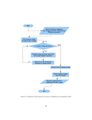
Leave-one-out cross-validation was used for testing the model. From n
healthy brain images, n − 1 were used as training images, and 1 was used for
testing. All AD brains were used as test images. This process was repeated n
times so that each image was used as a testing image once. Due to low amounts
of data (brain scans), this was necessary to get as many training images as
possible. The whole process from registration to prediction is summarized in
Figure 9.
3.3 Voxel-Based Morphometry
3.3.1 Prediction
Registered, segmented and eroded images were separated into training and test
sets. Like in the previous section, all non-common voxels were removed to ensure
that each brain had the same number of voxels (ncommon). For each image I in
the training set, Idx, Idy, and Idz were calculated as described in Section 2.2.1.
Three matrices X, Y , and Z were then formed such that
Xij = Ii
dx(j) = [x1, . . . , xncommon
] (31)
where Ii
refers to the ith image in the training set, and xj corresponds to the jth
column of X. X is then nimages ×ncommon. Each column contains x coordinate
displacements of one common voxel for all images. Y , Z, yj, and zj are defined
in a similar way. The columns of each matrix are normalized to have zero mean
and unit variance. The ages of the training set brains are stored in a nimages ×1
vector a. For matrix X linear correlation coefficients ρj and p-values pj were
calculated between each xj, and a. Linear regression using least squares was
also performed on xj and a to find functions fj for each voxel
Aβj = a (32)
βj = (AT
A)−1
AT
a (33)
where A = [xj, 1], and βj is a 2 × 1 vector that defines fj:
fj(dxj) = βj(1)dxj + βj(2) (34)
where dxj is a x displacement of the jth common brain voxel. βj, ρj, and pj
are saved for each voxel. This is done correspondingly for Y and Z.
21

27. Figure 9: Flowchart illustrating the whole process of using a morphable model
to predict brain ages.
22

28. To predict the age of a new image, it is first registered and non-common
voxels are deleted. From the registered image J, Jdx, Jdy and Jdz are calculated.
Each element in Jdx gives an age prediction fj(Jdx(j)). If pj is less than the
p-value threshold, then this prediction is labelled as significant. The prediction
is then the weighted sum of all significant predictions, where the weights are
ρ2
j . This done correspondingly for Jdy and Jdz. The total prediction is then the
average of the three. The p-value threshold used was 0.01. This algorithm was
implemented with leave-one-out cross-validation, same as with the morphable
model.
3.3.2 Analysis
The goal of this method is not prediction, but to see if there are any structural
differences between healthy and diseased brains. As in the previous subsection,
registered images are used and non-common voxels are removed. The images
are split into healthy and diseased sets. For each image, I, a displacement field
D is calculated. The displacement field is an image of the same size as I, whose
voxel values are displacement vectors. The displacement vector at the jth voxel
is
dj = [Idx(j), Idy(j), Idz(j)] = [dj,x, dj,y, dj,z] (35)
At each voxel of D, the Jacobian Determinant is calculated
JD = det



∂dx
∂dx
∂dx
∂dy
∂dx
∂dz
∂dy
∂dx
∂dy
∂dy
∂dy
∂dz
∂dz
∂dx
∂dz
∂dy
∂dz
∂dz


 (36)
where the voxel index j has been omitted for clarity. The Jacobian Determinant
represents local volume changes. Images are constructed where each voxel value
is the Jacobian Determinant, for each image in each set. For each set of JD
images, p-values are calculated for each voxel in the same way as the previous
section. The p-values are used to create yet another image where each voxel
value is the p-value. The result is two p-value images- one for the healthy set
and one for the diseased set. These can be compared either by visual inspection
or using an image similarity metric (section 2.1.1.1). The mean squares image
similarity metric was chosen to compare the images, because their values are in
the same range (p-values 0 to 1). Ten pairs of these images were created from
random subsets of 15 healthy and 15 AD images. Each of the 10 images in each
set was compared to each image in the same set, and all images in the other set.
Methods for calculating the JD image from a displacement field are imple-
mented in ITK.
23

29. 4 Results
4.1 Data Pre-Processing
Image Registration Figure 10 shows a sample brain image and the fixed
brain image before registration.
Figure 10: Fixed image (green) and a moving image (blue) before registration
with affine transform, along the z, x, and y axes. Brains are side by side on top,
and overlapped on the bottom.
Figure 11 shows the sample brain as the moving image and fixed brain image
image after affine registration. The fixed and moving brain images have roughly
the same shape, but the structure on the inside is different. After applying B-
spline registration, the brains have the same shape, and the structure on the
inside looks almost the same for both the moving and fixed brain images.
24

30. Figure 11: Fixed image (green) and a moving image (blue) after registration
with affine transform, along the z, x, and y axes. Brains are side by side on top,
and overlapped on the bottom.
Figure 12: Fixed image (green) and a moving image (blue) after registration
with B-Spline transform, along the z, x, and y axes. Brains are side by side on
top, and overlapped on the bottom.
25

31. Segmentation and Erosion Figure 13 shows the result of applying segmen-
tation to the fixed brain image (the common brain). CSF is highlighted in red
and is removed before erosion. Figure 14 shows the parts of the brain that are
left after CSF removal and erosion. The corresponding areas on a sample image
are calculated using the corresponding inverse B-spline transform on the fixed
image. Figure 15 compares the result with the fixed image.
Figure 13: Fixed image after segmentation. White corresponds to WM, gray to
GM and red to CSF
Figure 14: Fixed image after segmentation and erosion.
Figure 15: Fixed image after segmentation and erosion (left). Segmentation
and erosion of a sample image (right) calculated using the common segmented
image and an inverse B-spline transform.
26

32. 4.2 Morphable Model
The SVM regression parameters that were found to produce the best results
were
= 0.1
C = 10−15
c = 1
d = 3
npc = 30
(37)
The linear kernel d = 1 could not even classify the training data, therefore a 3rd
order kernel was used. The classification got better with higher npc, but with
only 60 training images (using cross validation) a maximum of 60 principal
components could be produced. As npc approached the number of training
samples, classification got worse again. determined the acceptable training
error, it was found that having this parameter low gave better results. The
results are presented in Figure 16 and Figure 17. The mean squared prediction
error was 41.0 years for healthy test data, and 59.2 years for AD test data. The
average predicted age was 72.85 years (stdev. 0.67) and 74.10 years (stdev 0.31)
for healthy and AD test brains, respectively.
4.3 Voxel-Based Morphometry
Prediction The results of VBM prediction are summarized in Figure 18 and
Figure 19. The mean squared prediction error was 34.9 years for healthy test
data, and 56.1 years for AD test data. The average predicted age was 75.47
years (stdev. 0.45) and 75.69 years (stdev 0.36) for healthy and AD test brains,
respectively.
27

33. Figure 16: Morphable model prediction using SVM re-
gression.
Figure 17: Whisker plot showing distributions of healthy
and AD predictions. t-test p-value 0.001
28

34. Figure 18: Morphable model prediction using SVM re-
gression.
Figure 19: Whisker plot showing distributions of healthy
and AD predictions. t-test p-value = 0.01
29

35. Analysis p-value images obtained from VBM are shown in Figure 20. Results
of comparing p-value images of both sets are in Table 4.3, and Figure 21.
Figure 20: p-value images produced by VBM. Top image obtained from healthy
brain image, bottom image from AD brain images
Same-Same Healthy-AD
Mean squared error
Mean (SD) 0.0277 (0.0028) 0.0320 (0.0005)
Table 3: Results of mean square comparison between different sets of Jaco-
bian determinant p-value images. Same-Same refers to the results of comparing
healthy to healthy and Healthy-AD to comparing healthy and AD sets.
30

36. Figure 21: Whisker plot illustrating the result of mean square comparison be-
tween different sets of Jacobian determinant p-value images. Same-Same refers
to the results of comparing healthy to healthy and Healthy-AD to comparing
healthy and AD sets. t-test p-value 0.001
31

37. 5 Conclusions and Discussion
Although the SVM regression was unable to predict brain age, the results pre-
sented in Figure 16 and Figure 17 show that it still consistently predicted AD
brain images to have a higher age than healthy brains. This means that it
can be used as a classifier. Figure 22 shows the Receiver Operating Charac-
teristic (ROC) curve produced by separating healthy and AD predictions with
a line. To compare the result to the related works in Table 1.1.3, the accu-
racy/sensitivity/specificity were calculated to be 94/97/92. This was achieved
using a smaller dataset however, with a larger dataset these numbers may be
lower. It is also worth noting that the SVM was never trained to classify healthy
and AD brain images, it was trained to predict age. The classification came nat-
urally. A summary of Table 1.1.3 with the results of this paper included can be
seen in Table 5 for convenience.
Figure 22: ROC curve for SVM regression classification. Area under the curve
is AUC = 0.98.
There are multiple explanations that could account for the lack of age pre-
dictive ability of the SVM regression. Perhaps there was not enough data; 60
training samples may not be enough. V. Blanz and T. Vetter (1999) [2] used
100 male and 100 female faces to train their morphable model. The methods
in Table 1.1.3 also used 100+ images of both healthy and AD brains. The data
also may need to be separated into males and females, as there are structural
differences between male and female brains [27], this could not be done in this
study due to the lack of data. Another problem with the data was that the
majority of healthy brain images were between 70 and 76 years old. Ideally the
data would be of a greater range of ages, with multiple samples of each age.
With more data, more principal components could also be calculated. Because
of the way PCA works, principal components hold structural information about
32

38. Article Data Result
Aguilar et al. (2013) [31] 116/110 88/86/90
Ewers et al. (2012) [28] 81/101 94/96/95
Nho et al. (2010) [33] 182/226 91/85/95
Spulber et al. (2013) [18] 295/335 88/86/90
Westman et al. (2013) [21] 187/225 92/90/93
This paper (Morphable Model) 35/61 94/97/92
Table 4: Summary of Table 1.1.3 with the results of this paper included.
Data shows number of AD/Healthy subjects in dataset. Results show accu-
racy/sensitivity/specificity for classification of healthy vs AD subjects.
the brain in descending order. The first few principal components describe the
big differences, while later principle components describe the more subtle fea-
tures of the brains. Perhaps age information is more of a subtle feature and is
present in the later principal components.
The results in Figure 18 and Figure 19 also show no predictive ability. There
is no significant difference between healthy and AD test data age predictions.
According to Good et al. (2001) [10], the results of voxel-based morphometry
may in some cases be heavily influenced by the registration method. This may
be the case here. The patterns in Figure 20 may be caused by the warpfield of
the B-spline transform. Figure 21 and Table 4.3 however shows that there is a
difference between p-value images created from healthy and AD brain images.
Both this result and the result from Figure 16 and Figure 17 seem to support
that there is information related to age/AD in the deformation fields created
by the B-Spline transforms.
6 Recommendations
The method based on Morphable Models is fast and compatible with low-quality
MRI brain images. This gives it an advantage over other methods. For future
work, it is recommended to have a larger and more varied data set to be able
to calculate more principal components. Also, testing with MCI-converter and
MCI-stable is necessary to further compare it to other methods. The expected
outcome would be a whisker plot as in Spulber et al. (2013) [18], Figure 23,
where MCI-converter and MCI-stable datasets would fall somewhere in between
the healthy and AD datasets. Another study could be done using CT brain
images. Because CT images are by far the most common, the ability to work
with them would be an achievement.
33

39. Figure 23: Classification results of different data sets. Source: [18]
34

40. References
[1] J. Ashburner; and K. J. Friston. Voxel–based morphometry—-the methods.
NeuroImage, 11:805–821, 2000.
[2] V. Blanz; and T. Vetter. A morphable model for the synthesis of 3d faces. In
Proc. of the 26th annual conference on Computer graphics and interactive
techniques, pages 187–194. ACM Press/Addison-Wesley Publishing Co.,
1999.
[3] M. Borda. Fundamentals in information theory and coding, volume 6.
Springer, 2011.
[4] S.M. Smith; M. Jenkinson; M.W. Woolrich; C.F. Beckmann; T.E.J.
Behrens; H. Johansen-Berg; P.R. Bannister; M. De Luca; I. Drobnjak; D.E.
Flitney; R. Niazy; J. Saunders; J. Vickers; Y. Zhang; N. De Stefano; J.M.
Brady; and P.M. Matthews. Advances in functional and structural mr
image analysis and implementation as fsl. NeuroImage, 23:208–219, 2004.
[5] Y. Zhang; M. Brady; and S. Smith. Segmentation of brain mr im-
ages through a hidden markov random field model and the expectation-
maximization algorithm. IEEE Trans Med Imag, 20(1):45–57, 2001.
[6] C. Chang; and C. Lin. LIBSVM: A library for support vector ma-
chines. ACM Transactions on Intelligent Systems and Technology, 2:27:1–
27:27, 2011. Software available at http://www.csie.ntu.edu.tw/~cjlin/
libsvm.
[7] C. Cortes; and V. Vapnik. Support-vector networks. Machine learning,
20(3):273–297, 1995.
[8] T. S. Curry; J. E. Dowdey; and R. C. Murry. Christensen’s physics of
diagnostic radiology. Lippincott Williams & Wilkins, 1990.
[9] A. Mechelli; C. J. Price; K. J. Friston; and J. Ashburner. Voxel-based
morphometry of the human brain: Methods and applications. Current
Medical Imaging Reviews, 1(1), 2005.
[10] C. D. Good; I. S. Johnsrude; J. Ashburner; R. N. A. Henson; K. J. Friston;
and R. S. J. Frackowiak. A voxel based morphometric study of ageing in
465 normal adult brains. NeuroImage, 14:21–36, 2001.
[11] P. A. Yushkevich; J. Piven; H. C. Hazlett; R. G. Smith; S. Ho; J. C. Gee;
and G. Gerig. User-guided 3D active contour segmentation of anatomical
structures: Significantly improved efficiency and reliability. Neuroimage,
31(3):1116–1128, 2006.
[12] H. J. Johnson; M. McCormick; L. Ib´a˜nez; and The Insight Software Con-
sortium. The ITK Software Guide. Kitware, Inc., third edition, 2013. In
press. URL: http://www.itk.org/ItkSoftwareGuide.pdf.
35

41. [13] M.W. Woolrich; S. Jbabdi; B. Patenaude; M. Chappell; S. Makni; T.
Behrens; C. Beckmann; M. Jenkinson; and S.M. Smith. Bayesian anal-
ysis of neuroimaging data in fsl. NeuroImage, 45:173–186, 2009.
[14] K. Held; E. R. Kops; B. J. Krause; W. M. I. I. I. Wells; R. Kikinis; and H-
W Muller-Gartner. Markov random field segmentation of brain mr images.
Medical Imaging, IEEE Transactions on, 16(6):878–886, 1997.
[15] D. Rueckert; L. I. Sonoda; C. Hayes; D. L. G. Hill; M. O. Leach; and D. J.
Hawkes. Nonrigid registration using free-form deformations: Application to
breast mr images. IEEE Transaction on Medical Imaging, 18(8):712—-721,
1999.
[16] D. Mattes; D. R. Haynor; H. Vesselle; T. K. Lewellen; and W. Eubank.
Non-rigid multimodality image registration. In Proc. of Medical Imaging
2001: Image Processing, pages 1609––1620, 2001.
[17] D. Mattes; D. R. Haynor; H. Vesselle; T. K. Lewellen; and W. Eubank.
Pet-ct image registration in the chest using free-form deformations. IEEE
Trans. on Medical Imaging, 22(1):120––128, January 2003.
[18] G. Spulber; A. Simmons; J-S. Muehlboeck; P. Mecocci; B. Vellas; M. Tso-
laki; I. Kloszewska; H. Soininen; C. Spenger; S. Lovestone; et al. An mri-
based index to measure the severity of alzheimer’s disease-like structural
pattern in subjects with mild cognitive impairment. Journal of internal
medicine, 273(4):396–409, 2013.
[19] C. Zhu; R. H. Byrd; P. Lu; and J. Nocedal. Algorithm 778: L-bfgs-b:
Fortran subroutines for large-scale bound-constrained optimization. ACM
Transactions on Mathematical Software (TOMS), 23(4):550–560, 1997.
[20] T. S. Yoo; M. J. Ackerman; W. E. Lorensen; W. Schroeder; V. Chalana;
S. Aylward; D. Metaxas; and R. Whitaker. Engineering and algorithm
design for an image processing api: A technical report on itk - the insight
toolkit. In Proc. of Medicine Meets Virtual Reality, J. Westwood, ed., pages
586–592. IOS Press Amsterdam, 2002.
[21] E. Westman; C. Aguilar; J-S. Muehlboeck; and A. Simmons. Regional mag-
netic resonance imaging measures for multivariate analysis in alzheimer’s
disease and mild cognitive impairment. Brain topography, 26(1):9–23, 2013.
[22] J. Dukart; M. L. Schroeter; K. Mueller;, Alzheimer’s Disease Neuroimaging
Initiative, et al. Age correction in dementia–matching to a healthy brain.
PloS one, 6(7):e22193, 2011.
[23] R. H. Byrd; P. Lu; J. Nocedal; and C. Zhu. A limited memory algorithm for
bound constrained optimization. SIAM Journal on Scientific Computing,
16(5):1190–1208, 1995.
36

42. [24] G. McKhann; D. Drachman; M. Folstein; R. Katzman; D. Price; and E. M.
Stadlan. Clinical diagnosis of alzheimer’s disease report of the nincds-adrda
work group* under the auspices of department of health and human services
task force on alzheimer’s disease. Neurology, 34(7):939–939, 1984.
[25] A. Wimo; L. J¨onsson; J. Bond; M. Prince; and B. Winblad. The worldwide
economic impact of dementia 2010. Alzheimer’s & Dementia, 9(1):1–11,
2013.
[26] M. Rosenblatt; et al. Remarks on some nonparametric estimates of a den-
sity function. The Annals of Mathematical Statistics, 27(3):832–837, 1956.
[27] Amber NV Ruigrok, Gholamreza Salimi-Khorshidi, Meng-Chuan Lai, Si-
mon Baron-Cohen, Michael V Lombardo, Roger J Tait, and John Suckling.
A meta-analysis of sex differences in human brain structure. Neuroscience
& Biobehavioral Reviews, 39:34–50, 2014.
[28] M. Ewers; C. Walsh; J. Q. Trojanowski; L. M. Shaw; R. C. Petersen; C.
R. Jack Jr; H. H. Feldman; A. L. W. Bokde; G. E. Alexander; P. Schel-
tens; et al. Prediction of conversion from mild cognitive impairment to
alzheimer’s disease dementia based upon biomarkers and neuropsychologi-
cal test performance. Neurobiology of aging, 33(7):1203–1214, 2012.
[29] A. J. Smola; and B. Sch¨olkopf. A tutorial on support vector regression.
Statistics and computing, 14(3):199–222, 2004.
[30] H. Drucker; Christopher J. C. Burges; L. Kaufman; A. J. Smola; and
V. Vapnik. Support vector regression machines. In Proc. of Advances
in Neural Information Processing Systems 9, pages 155—-161. MIT Press,
1997.
[31] C. Aguilar; E. Westman; J. Muehlboeck; P. Mecocci; B. Vellas; M. Tsolaki;
I. Kloszewska; H. Soininen; S. Lovestone; C. Spenger; et al. Different mul-
tivariate techniques for automated classification of mri data in alzheimer’s
disease and mild cognitive impairment. Psychiatry Research: Neuroimag-
ing, 212(2):89–98, 2013.
[32] J. B. Pereira; L. Cavallin; G. Spulber; C. Aguilar; P. Mecocci; B. Vellas;
M. Tsolaki; I. Kloszewska; H. Soininen; C. Spenger; et al. Influence of age,
disease onset and apoe4 on visual medial temporal lobe atrophy cut-offs.
Journal of internal medicine, 275(3):317–330, 2014.
[33] K. Nho; L. Shen; S. Kim; S. L. Risacher; J. D. West; T. Foroud; C. R.
Jack Jr; M. W. Weiner; and A. J. Saykin. Automatic prediction of con-
version from mild cognitive impairment to probable alzheimer’s disease
using structural magnetic resonance imaging. In AMIA Annual Sympo-
sium Proceedings, volume 2010, page 542. American Medical Informatics
Association, 2010.
37

43. [34] F. Falahati; E. Westman; and A. Simmons. Multivariate data analysis and
machine learning in alzheimer’s disease with a focus on structural magnetic
resonance imaging. Journal of Alzheimer’s Disease, 2014.
[35] F. Falahati; S-M. Fereshtehnejad; D. Religa; L-O. Wahlund; E. Westman;
and M. Eriksdotter. The use of mri, ct and lumbar puncture in demen-
tia diagnostics: Data from the svedem registry. Dementia and geriatric
cognitive disorders, 39(1-2):81–91, 2015.
[36] S. Damangir; A. Manzouri; K. Oppedal; S. Carlsson; M. J. Firbank; H.
Sonnesyn; O-B. Tysnes; J. T. O’Brien; M. K. Beyer; E. Westman; et al.
Multispectral mri segmentation of age related white matter changes using
a cascade of support vector machines. Journal of the neurological sciences,
322(1):211–216, 2012.
[37] M. Jenkinson; C.F. Beckmann; T.E. Behrens; M.W. Woolrich; and S.M.
Smith. Fsl. Neuroimage, 62:782–790, 2012.
38

44. Appendix
Let X be a matrix. Define:
C = XX (38)
C1 = X X (39)
Let C1 have an eigenvalue L1 and eigenvector v1 such that:
C1v1 = L1v1 (40)
Substitute 39 into 40:
X Xv1 = L1v1 (41)
Let
vx = Xv1 (42)
Rewrite 41 using 42:
X vx = L1v1 (43)
Multiply 43 by X:
XX vx = L1Xv1 (44)
Using 42:
XX vx = L1vx (45)
Using 38:
Cvx = L1vx (46)
⇒ vx is an eigenvector of C.
39

45. www.kth.se