Downloaded 15 times


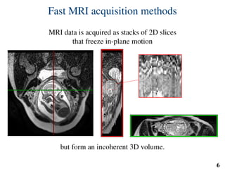

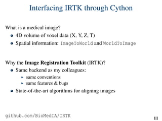

![Implementation: training
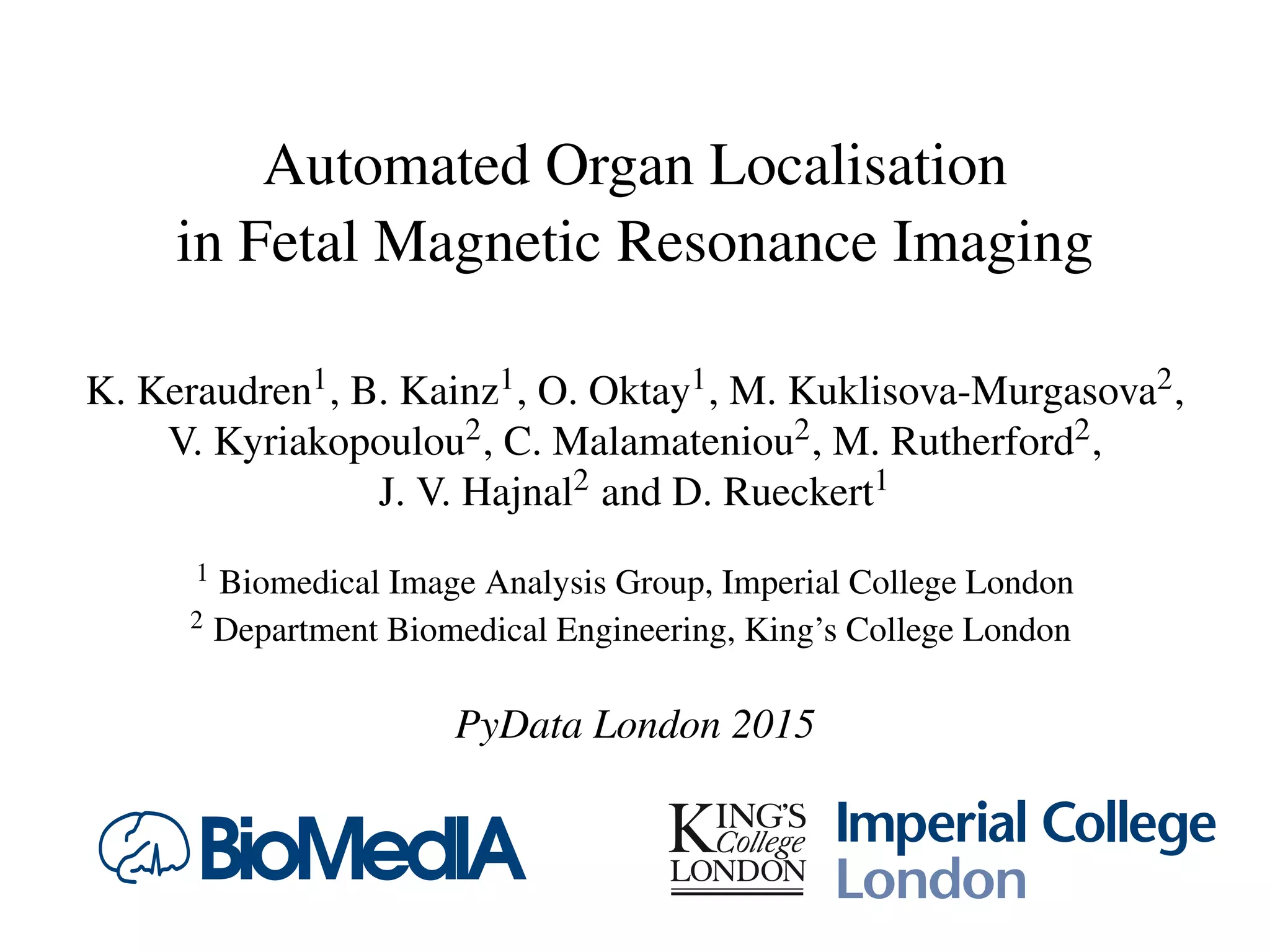
# predefined set of cube features
offsets = np.random.randint( -o_size, o_size+1, size=(n_tests,3) )
sizes = np.random.randint( 0, d_size+1, size=(n_tests,1) )
X = []
Y = []
for l in range(nb_labels):
pixels = np.argwhere(np.logical_and(narrow_band>0,seg==l))
pixels = pixels[np.random.randint( 0,
pixels.shape[0],
n_samples)]
u,v,w = get_orientation_training( pixels, organ_centers )
x = extract_features( pixels, w, v, u )
y = seg[pixels[:,0],
pixels[:,1],
pixels[:,2]]
X.extend(x)
Y.extend(y)
clf = RandomForestClassifier(n_estimators=100) # scikit-learn
clf.fit(X,Y)
47](https://image.slidesharecdn.com/presentation-150621183046-lva1-app6891/85/PyData-London-2015-Localising-Organs-of-the-Fetus-in-MRI-Data-Using-Python-61-320.jpg)
![Implementation: training
# predefined set of cube features
offsets = np.random.randint( -o_size, o_size+1, size=(n_tests,3) )
sizes = np.random.randint( 0, d_size+1, size=(n_tests,1) )
X = []
Y = []
for l in range(nb_labels):
pixels = np.argwhere(np.logical_and(narrow_band>0,seg==l))
pixels = pixels[np.random.randint( 0,
pixels.shape[0],
n_samples)]
u,v,w = get_orientation_training( pixels, organ_centers )
x = extract_features( pixels, w, v, u )
y = seg[pixels[:,0],
pixels[:,1],
pixels[:,2]]
X.extend(x)
Y.extend(y)
clf = RandomForestClassifier(n_estimators=100) # scikit-learn
clf.fit(X,Y)
47](https://image.slidesharecdn.com/presentation-150621183046-lva1-app6891/85/PyData-London-2015-Localising-Organs-of-the-Fetus-in-MRI-Data-Using-Python-62-320.jpg)
![Implementation: training
# predefined set of cube features
offsets = np.random.randint( -o_size, o_size+1, size=(n_tests,3) )
sizes = np.random.randint( 0, d_size+1, size=(n_tests,1) )
X = []
Y = []
for l in range(nb_labels):
pixels = np.argwhere(np.logical_and(narrow_band>0,seg==l))
pixels = pixels[np.random.randint( 0,
pixels.shape[0],
n_samples)]
u,v,w = get_orientation_training( pixels, organ_centers )
x = extract_features( pixels, w, v, u )
y = seg[pixels[:,0],
pixels[:,1],
pixels[:,2]]
X.extend(x)
Y.extend(y)
clf = RandomForestClassifier(n_estimators=100) # scikit-learn
clf.fit(X,Y)
47](https://image.slidesharecdn.com/presentation-150621183046-lva1-app6891/85/PyData-London-2015-Localising-Organs-of-the-Fetus-in-MRI-Data-Using-Python-63-320.jpg)
![Implementation: training
# predefined set of cube features
offsets = np.random.randint( -o_size, o_size+1, size=(n_tests,3) )
sizes = np.random.randint( 0, d_size+1, size=(n_tests,1) )
X = []
Y = []
for l in range(nb_labels):
pixels = np.argwhere(np.logical_and(narrow_band>0,seg==l))
pixels = pixels[np.random.randint( 0,
pixels.shape[0],
n_samples)]
u,v,w = get_orientation_training( pixels, organ_centers )
x = extract_features( pixels, w, v, u )
y = seg[pixels[:,0],
pixels[:,1],
pixels[:,2]]
X.extend(x)
Y.extend(y)
clf = RandomForestClassifier(n_estimators=100) # scikit-learn
clf.fit(X,Y)
47](https://image.slidesharecdn.com/presentation-150621183046-lva1-app6891/85/PyData-London-2015-Localising-Organs-of-the-Fetus-in-MRI-Data-Using-Python-64-320.jpg)
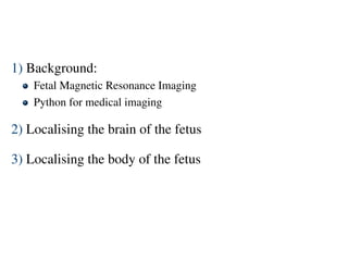
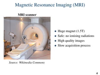
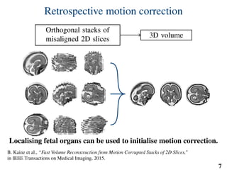
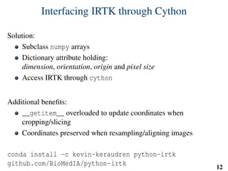
![Implementation: testing
def get_orientation( brain, pixels ):
u = brain - pixels
u /= np.linalg.norm( u, axis=1 )[...,np.newaxis]
# np.random.rand() returns random floats in the interval [0;1[
v = 2*np.random.rand( pixels.shape[0], 3 ) - 1
v -= (v*u).sum(axis=1)[...,np.newaxis]*u
v /= np.linalg.norm( v,
axis=1 )[...,np.newaxis]
w = np.cross( u, v )
# u and v are perpendicular unit vectors
# so ||w|| = 1
return u, v, w
Brain
Pixel
u
v
w
48](https://image.slidesharecdn.com/presentation-150621183046-lva1-app6891/85/PyData-London-2015-Localising-Organs-of-the-Fetus-in-MRI-Data-Using-Python-65-320.jpg)
![Implementation: testing
def get_orientation( brain, pixels ):
u = brain - pixels
u /= np.linalg.norm( u, axis=1 )[...,np.newaxis]
# np.random.rand() returns random floats in the interval [0;1[
v = 2*np.random.rand( pixels.shape[0], 3 ) - 1
v -= (v*u).sum(axis=1)[...,np.newaxis]*u
v /= np.linalg.norm( v,
axis=1 )[...,np.newaxis]
w = np.cross( u, v )
# u and v are perpendicular unit vectors
# so ||w|| = 1
return u, v, w
Brain
Pixel
u
v
w
48](https://image.slidesharecdn.com/presentation-150621183046-lva1-app6891/85/PyData-London-2015-Localising-Organs-of-the-Fetus-in-MRI-Data-Using-Python-66-320.jpg)
![Implementation: testing
def get_orientation( brain, pixels ):
u = brain - pixels
u /= np.linalg.norm( u, axis=1 )[...,np.newaxis]
# np.random.rand() returns random floats in the interval [0;1[
v = 2*np.random.rand( pixels.shape[0], 3 ) - 1
v -= (v*u).sum(axis=1)[...,np.newaxis]*u
v /= np.linalg.norm( v,
axis=1 )[...,np.newaxis]
w = np.cross( u, v )
# u and v are perpendicular unit vectors
# so ||w|| = 1
return u, v, w
Brain
Pixel
u
v
w
48](https://image.slidesharecdn.com/presentation-150621183046-lva1-app6891/85/PyData-London-2015-Localising-Organs-of-the-Fetus-in-MRI-Data-Using-Python-67-320.jpg)
![Implementation: testing
def get_orientation( brain, pixels ):
u = brain - pixels
u /= np.linalg.norm( u, axis=1 )[...,np.newaxis]
# np.random.rand() returns random floats in the interval [0;1[
v = 2*np.random.rand( pixels.shape[0], 3 ) - 1
v -= (v*u).sum(axis=1)[...,np.newaxis]*u
v /= np.linalg.norm( v,
axis=1 )[...,np.newaxis]
w = np.cross( u, v )
# u and v are perpendicular unit vectors
# so ||w|| = 1
return u, v, w
Brain
Pixel
u
v
w
48](https://image.slidesharecdn.com/presentation-150621183046-lva1-app6891/85/PyData-London-2015-Localising-Organs-of-the-Fetus-in-MRI-Data-Using-Python-68-320.jpg)
![Implementation: testing
def get_orientation( brain, pixels ):
u = brain - pixels
u /= np.linalg.norm( u, axis=1 )[...,np.newaxis]
# np.random.rand() returns random floats in the interval [0;1[
v = 2*np.random.rand( pixels.shape[0], 3 ) - 1
v -= (v*u).sum(axis=1)[...,np.newaxis]*u
v /= np.linalg.norm( v,
axis=1 )[...,np.newaxis]
w = np.cross( u, v )
# u and v are perpendicular unit vectors
# so ||w|| = 1
return u, v, w
Brain
Pixel
u
v
w
48](https://image.slidesharecdn.com/presentation-150621183046-lva1-app6891/85/PyData-London-2015-Localising-Organs-of-the-Fetus-in-MRI-Data-Using-Python-69-320.jpg)
![Implementation: testing
def get_orientation( brain, pixels ):
u = brain - pixels
u /= np.linalg.norm( u, axis=1 )[...,np.newaxis]
# np.random.rand() returns random floats in the interval [0;1[
v = 2*np.random.rand( pixels.shape[0], 3 ) - 1
v -= (v*u).sum(axis=1)[...,np.newaxis]*u
v /= np.linalg.norm( v,
axis=1 )[...,np.newaxis]
w = np.cross( u, v )
# u and v are perpendicular unit vectors
# so ||w|| = 1
return u, v, w
Brain
Pixel
u
v
w
48](https://image.slidesharecdn.com/presentation-150621183046-lva1-app6891/85/PyData-London-2015-Localising-Organs-of-the-Fetus-in-MRI-Data-Using-Python-70-320.jpg)
![Implementation: testing
def get_orientation( brain, pixels ):
u = brain - pixels
u /= np.linalg.norm( u, axis=1 )[...,np.newaxis]
# np.random.rand() returns random floats in the interval [0;1[
v = 2*np.random.rand( pixels.shape[0], 3 ) - 1
v -= (v*u).sum(axis=1)[...,np.newaxis]*u
v /= np.linalg.norm( v,
axis=1 )[...,np.newaxis]
w = np.cross( u, v )
# u and v are perpendicular unit vectors
# so ||w|| = 1
return u, v, w
Brain
Pixel
u
v
w
48](https://image.slidesharecdn.com/presentation-150621183046-lva1-app6891/85/PyData-London-2015-Localising-Organs-of-the-Fetus-in-MRI-Data-Using-Python-71-320.jpg)
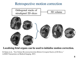
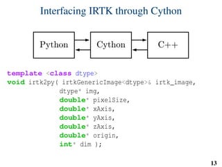
![Implementation: testing
img = irtk.imread(...) # Python interface to IRTK
proba = irtk.zeros(img.get_header(),dtype=’float32’)
...
pixels = np.argwhere(narrow_band>0)
u,v,w = get_orientation(brain_center,pixels)
# img is 3D so all features cannot fit in memory at once:
# use chunks
for i in xrange(0,pixels.shape[0],chunk_size):
j = min(i+chunk_size,pixels.shape[0])
x = extract_features( pixels[i:j],w[i:j],v[i:j],u[i:j])
pr = clf_heart.predict_proba(x)
for dim in xrange(nb_labels):
proba[dim,
pixels[i:j,0],
pixels[i:j,1],
pixels[i:j,2]] = pr[:,dim]
49](https://image.slidesharecdn.com/presentation-150621183046-lva1-app6891/85/PyData-London-2015-Localising-Organs-of-the-Fetus-in-MRI-Data-Using-Python-72-320.jpg)
![Implementation: testing
img = irtk.imread(...) # Python interface to IRTK
proba = irtk.zeros(img.get_header(),dtype=’float32’)
...
pixels = np.argwhere(narrow_band>0)
u,v,w = get_orientation(brain_center,pixels)
# img is 3D so all features cannot fit in memory at once:
# use chunks
for i in xrange(0,pixels.shape[0],chunk_size):
j = min(i+chunk_size,pixels.shape[0])
x = extract_features( pixels[i:j],w[i:j],v[i:j],u[i:j])
pr = clf_heart.predict_proba(x)
for dim in xrange(nb_labels):
proba[dim,
pixels[i:j,0],
pixels[i:j,1],
pixels[i:j,2]] = pr[:,dim]
49](https://image.slidesharecdn.com/presentation-150621183046-lva1-app6891/85/PyData-London-2015-Localising-Organs-of-the-Fetus-in-MRI-Data-Using-Python-73-320.jpg)
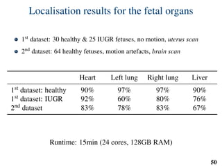


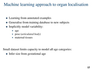
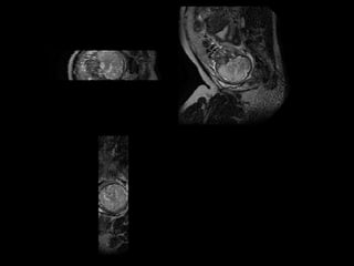
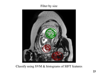
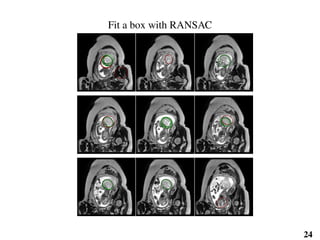
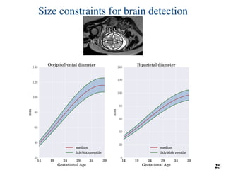
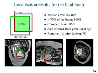
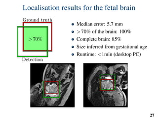
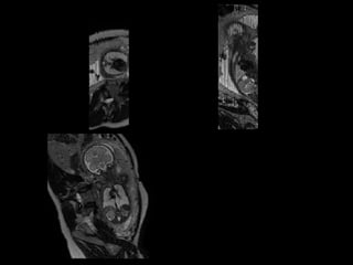
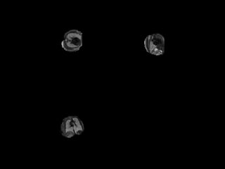
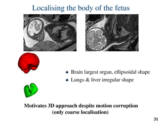
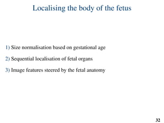
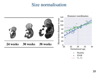
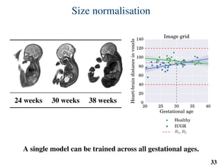
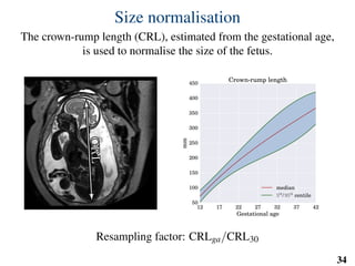
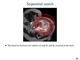
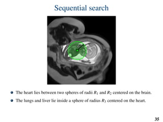
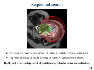
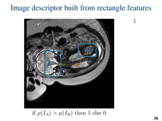
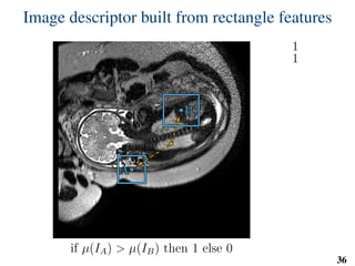
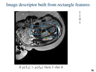
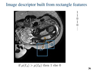
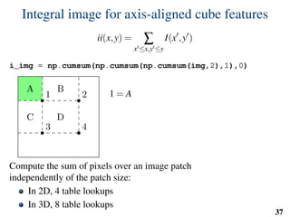
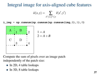
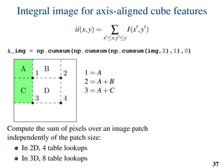
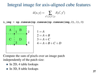
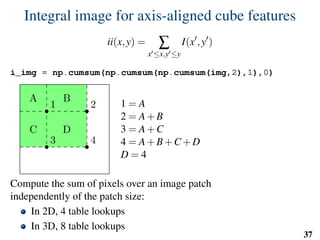
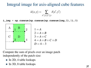
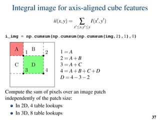
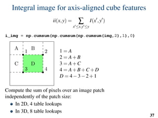
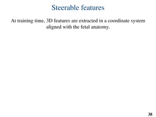
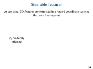
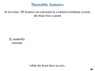
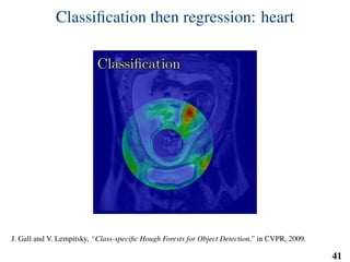
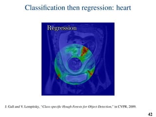
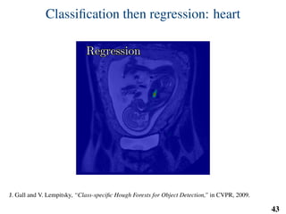
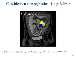
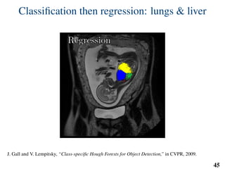
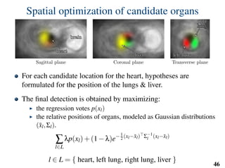
This document summarizes an automated method for localizing fetal organs in magnetic resonance images. The method uses machine learning to sequentially localize the brain, heart, lungs and liver. It first normalizes fetal size based on gestational age. It then localizes the brain, uses this to search for the heart between two spheres. The heart location guides searching inside a third sphere for the lungs and liver. Features incorporate spatial relationships modeled by Gaussian distributions. Classification predicts organ candidates, regression refines locations, and spatial optimization selects the final detection by maximizing votes and relative organ positions. Training involves extracting random cube features around labeled pixels to classify organs.


![Polymer [ बहुलक ] Chemistry Notes PDF - Irfanullah Mehar - JJ Sir Chemistry.pdf](https://cdn.slidesharecdn.com/ss_thumbnails/polymerchemistrynotespdf-irfanullahmehar-jjsirchemistry-260210172118-3f9b37f7-thumbnail.jpg?width=640&height=640&fit=bounds)

