The document describes a study that used convolutional neural networks (CNNs) to detect brain tumors in MRI images. Three CNN models were developed and their performance was evaluated using metrics like accuracy, precision, recall, F1-score, and confusion matrices. Model 3 achieved the highest test accuracy of 94% for tumor detection. In total, over 2000 MRI images were used in the study after data augmentation. The CNN models incorporated convolution, pooling, and fully connected layers to analyze image features and classify tumors. This research demonstrates that CNNs can accurately detect brain tumors in medical images.

1. Brain Tumor Detection using CNN
Drubojit Saha
170104027@aust.edu
Mohammad Rakib-Uz-Zaman
170104041@aust,edu
Tasnim Nusrat Hasan
170104046@aust.edu
Abstract—Diagnosis of brain tumors is an essential task in the
medical field for finding out if the tumor can probably become
cancerous. Deep learning is a convenient and decisive approach
for image classification. It has been broadly applied in diverse
fields like medical imaging, as its application does not require the
reliability of a skilled in the related field, but rather requires the
number of data and distinct data to produce good classification
conclusions. Convolutional Neural Network (CNN) is used for
image classification as well as recognized because of its immense
accuracy. In this paper, a comparison between two models of
CNN of our selected paper is shown to find the best model
to classify tumors in Brain MRI Image and at last, another
approach of a CNN model is trained and gained a prediction
accuracy of up to 94%.
I. INTRODUCTION
Medical imaging invokes a number of techniques that can
be used as non-interfering methods of looking inside the
body. Medical image compasses various image modalities
and converts to image of the human body for analyzing and
investigating purposes and thus it plays a great and decisive
role in taking actions for the enhancement of people’s health.
Image segmentation is an essential stride in image process-
ing which actuates the accomplishment of a higher level of
image processing. The fundamental goal of image segmenta-
tion in medical image processing is mainly detecting tumors,
competent machine vision and gaining satisfactory result for
further diagnosis.
Brain, as well as other nervous system cancer, is the 10th
leading reason of death and the five-year endurance rate for
people with a cancerous brain is 34 percent for men on
the other hand 36 percent for women. The World Health
Organization (WHO) states that around 400,000 people around
the world are affected by the brain tumor and 120,000 people
have died in the recent years.
Early detection of brain tumors has played an imperative
role in developing the treatment possibilities, and a higher
gain of survival possibility can be achieved. Although manual
segmentation of tumors is a tedious, challenging, and difficult
task as it requires a large number of MRI images that are
generated in medical routine. Magnetic Resonance Imaging
is mainly used for brain tumor detection. Brain tumor seg-
mentation from MRI is one of the most compelling tasks in
medical image processing as it involves a considerable amount
of data. Furthermore, the tumors can be ill-defined with soft
tissue boundaries. As a result, it is a very comprehensive task
Fig. 1. Dummy Input and Output of Proposed System
to gain the accurate segmentation of tumors from the human
brain.
II. RELATED WORKS
In [1] an achievement of substantial results in image
segmentation and classification is shown through the
convolutional neural network (CNN). A new CNN architecture
for brain tumor classification network is simpler than
already-existing pre-trained networks, and it was tested on
contrast-enhanced magnetic resonance images.
In [2] they have established the whole segmentation process
based on Mathematical Morphological Operations and applied
spatial FCM algorithm which improves the computation time.
In [3] they have established that Convolutional Neural
Networks are good enough to diagnose brain tumors on MRI
images. This study resulted in accuracy of 93% and a loss
value of 0.23264. The amount of convolution layers that
affects the quality of classification, more convolution layers
rise the accuracy results, but more convolution layers will
require more time for training.
III. OBJECTIVE
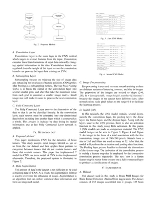
Convolutional Neural Networks are widely used in the
medical field for image processing. Over the years lots after
trying researchers built a model which can detect the tumor
more accurately. In this paper, the same idea has come up
which can accurately identify the tumor from Brain MRI
images. A fully connected neural network layer can detect the
tumor, but due to parameter sharing and sparsity of connection,
CNN is used as our model. The dummy figure of CNN is
shown in Figure 1.

2. Fig. 2. Proposed Method
A. Convolution Layer
Convolution Layer is the main layer in the CNN method
which targets to extract features from the input. Convolution
executes linear transformations of input data outwardly chang-
ing spatial information in the data. Convolution kernels are
regulated from the weight of the layer in case the convolution
kernels can process the input data training on CNN.
B. Subsampling Layer
Subsampling focuses on reducing the size of image data
and enhancing the invariance of feature positions. CNN applies
Max Pooling as a subsampling method. The way Max Pooling
works is to break the output of the convolution layer into
several smaller grids and after that take the maximum value
from each grid to construct a smaller image matrix. Small
image size will make it easier to process the next convolution
layer
C. Fully Connected Layer
The Fully Connected Layer evolves the dimensions of the
data so that it can be classified linearly. In the convolution
layer, each neuron must be converted into one-dimensional
data before including into another layer which is connected as
a whole. This process is induced by data losing its spatial
information and at last Fully Connected Layer network is
applied.
IV. METHODOLOGY
A. Proposed Method
This paper implements CNN for the detection of brain
tumors. This study accepts input images labeled as yes or
no from the raw dataset and then applies these patterns to
categorize between tissues that do not contain tumors and
those that contain tumors. This paper has implemented 2
model for CNN. An extra model of CNN is also implemented
afterwards. Therefore, the proposed system is illustrated in
Figure 2.
B. Data Augmentation
The amount of data in the dataset is not sufficient to be used
as training data for CNN. As a result, the augmentation method
is used to overcome the imbalance of issues. Augmentation is
an algorithm that can utilize statistical data information and
form an integrated model.
Fig. 3. First CNN Model
Fig. 4. Second CNN Model
C. Image Pre-processing
Pre-processing is executed to create smooth training as there
are different variants of intensity, contrast, and size in images.
The proportion of the images are resized to shape (240,
240, 3) = (imagewidth, imageheight, numberofchannels)
because the images in the dataset have different sizes. After
normalization, scale pixel values to the range 0-1 to facilitate
the learning process.
D. Model CNN
In this research, the CNN model contains several layers,
namely the convolution layer, the pooling layer, the dense
layer, the flatten layer, and the dropout layer. Along with the
layers used in the CNN process, there is also an activation
function in this study using Relu activation. In this paper,
3 CNN models are made as comparison material. The CNN
model design can be seen in Figure 3, Figure 4 and Figure
5. An image in the form of a total association with the first
convolution, image size of 240x240 pixels. Kernels have a
size of 3x3 and filters are used as many as 32. After that, the
model will perform the activation and pooling data functions.
The Pooling layer process handles to diminish the dimensions
of the feature map. The derivation of the convolution process
is mainly a feature map that is employed for the consecutive
convolution process repeatedly. The next step is a flatten
feature map in vector form to carry out a fully connected layer
to produce a classification of images.
V. EXPERIMENTS
A. Dataset
The dataset used in this study is Brain MRI Images for
Brain Tumor Detection obtained from kaggle.com. The dataset
consists of 253 images assembled into 2 groups, 155 brain

3. Fig. 5. Third CNN Model
Fig. 6. First Image without having any Tumor and Second Image having a
Brain Tumor
images that have tumors, and the rest 98 brain images that
do not have tumors. After data augmentation, the dataset
subsists of 1085 samples containing tumors and 980 samples
not containing tumors, bringing a total of 2065 images. The
images having tumor and no tumor is shown in Figure 6. The
dataset is splitted into training, testing and validation set with
70:15:15 ratio.
B. Evaluation Metrices
The evaluation matrices for the three model are repre-
sented by Classification Report(Accuracy, Precision, Recall,
F1-score), Confusion Matrix as well as Loss Curve.
1) CNN Model 1: For Model 1 the evaluation matrices are
shown in Figure 7. Figure 8, Figure 9. Figure 10, Figure 11.
Figure 12, Figure 13. Figure 14, Figure 15. Figure 16, Figure
17. Figure 18, Figure 19. Figure 20, Figure 21. Figure 22,
Figure 23. Figure 24, Figure 25. Figure 26.
Fig. 7. Confusion Matrix and Loss Curve of Model 1 (Run 1)
Fig. 8. Classification Report of Model 1 (Run 1)
Fig. 9. Confusion Matrix and Loss Curve of Model 1 (Run 2)
Fig. 10. Classification Report of Model 1 (Run 2)
Fig. 11. Confusion Matrix and Loss Curve of Model 1 (Run 3)
Fig. 12. Classification Report of Model 1 (Run 3)
Fig. 13. Confusion Matrix and Loss Curve of Model 1 (Run 4)
Fig. 14. Classification Report of Model 1 (Run 4)
Fig. 15. Confusion Matrix and Loss Curve of Model 1 (Run 5)

4. Fig. 16. Classification Report of Model 1 (Run 5)
Fig. 17. Confusion Matrix and Loss Curve of Model 1 (Run 6)
Fig. 18. Classification Report of Model 1 (Run 6)
Fig. 19. Confusion Matrix and Loss Curve of Model 1 (Run 7)
Fig. 20. Classification Report of Model 1 (Run 7)
Fig. 21. Confusion Matrix and Loss Curve of Model 1 (Run 8)
2) CNN Model 2: For Model 2, the evaluation matrices are
shown in Figure 27. Figure 28, Figure 29. Figure 30, Figure
31. Figure 32, Figure 33. Figure 34, Figure 35. Figure 36,
Figure 37. Figure 38, Figure 39. Figure 40, Figure 41. Figure
42, Figure 43. Figure 44, Figure 45. Figure 46.
3) CNN Model 3: For Model 2, the evaluation matrices are
shown in Figure 47. Figure 48, Figure 49. Figure 50, Figure
Fig. 22. Classification Report of Model 1 (Run 8)
Fig. 23. Confusion Matrix and Loss Curve of Model 1 (Run 9)
Fig. 24. Classification Report of Model 1 (Run 9)
Fig. 25. Confusion Matrix and Loss Curve of Model 1 (Run 10)
Fig. 26. Classification Report of Model 1 (Run 10)
Fig. 27. Confusion Matrix and Loss Curve of Model 2 (Run 1)
Fig. 28. Classification Report of Model 2 (Run 1)

5. Fig. 29. Confusion Matrix and Loss Curve of Model 2 (Run 2)
Fig. 30. Classification Report of Model 2 (Run 2)
Fig. 31. Confusion Matrix and Loss Curve of Model 2 (Run 3)
Fig. 32. Classification Report of Model 2 (Run 3)
Fig. 33. Confusion Matrix and Loss Curve of Model 2 (Run 4)
Fig. 34. Classification Report of Model 2 (Run 4)
Fig. 35. Confusion Matrix and Loss Curve of Model 2 (Run 5)
Fig. 36. Classification Report of Model 2 (Run 5)
Fig. 37. Confusion Matrix and Loss Curve of Model 2 (Run 6)
Fig. 38. Classification Report of Model 2 (Run 6)
Fig. 39. Confusion Matrix and Loss Curve of Model 2 (Run 7)
Fig. 40. Classification Report of Model 2 (Run 7)
Fig. 41. Confusion Matrix and Loss Curve of Model 2 (Run 8)
Fig. 42. Classification Report of Model 2 (Run 8)

6. Fig. 43. Confusion Matrix and Loss Curve of Model 2 (Run 9)
Fig. 44. Classification Report of Model 2 (Run 9)
Fig. 45. Confusion Matrix and Loss Curve of Model 2 (Run 10)
Fig. 46. Classification Report of Model 2 (Run 10)
51. Figure 52, Figure 53. Figure 54, Figure 55. Figure 56,
Figure 57. Figure 58, Figure 59. Figure 60, Figure 61. Figure
62, Figure 63. Figure 64, Figure 65. Figure 66.
Fig. 47. Confusion Matrix and Loss Curve of Model 3 (Run 1)
Fig. 48. Classification Report of Model 3 (Run 1)
Fig. 49. Confusion Matrix and Loss Curve of Model 3 (Run 2)
Fig. 50. Classification Report of Model 3 (Run 2)
Fig. 51. Confusion Matrix and Loss Curve of Model 3 (Run 3)
Fig. 52. Classification Report of Model 3 (Run 3)
Fig. 53. Confusion Matrix and Loss Curve of Model 3 (Run 4)
Fig. 54. Classification Report of Model 3 (Run 4)
Fig. 55. Confusion Matrix and Loss Curve of Model 3 (Run 5)

7. Fig. 56. Classification Report of Model 3 (Run 5)
Fig. 57. Confusion Matrix and Loss Curve of Model 3 (Run 6)
Fig. 58. Classification Report of Model 3 (Run 6)
Fig. 59. Confusion Matrix and Loss Curve of Model 3 (Run 7)
Fig. 60. Classification Report of Model 3 (Run 7)
Fig. 61. Confusion Matrix and Loss Curve of Model 3 (Run 8)
C. Results
Experiments in this article are carried out on 2065 images
consisting of 1085 samples containing tumors and 980 samples
containing no tumors. The data has been run for 10 times,
each using the CNN model that has been made before, each
experiment using 25 epochs and 32 batches.
Fig. 62. Classification Report of Model 3 (Run 8)
Fig. 63. Confusion Matrix and Loss Curve of Model 3 (Run 9)
Fig. 64. Classification Report of Model 3 (Run 9)
Fig. 65. Confusion Matrix and Loss Curve of Model 3 (Run 10)
Fig. 66. Classification Report of Model 3 (Run 10)
1) CNN Model 1: This model gives highest training accu-
racy value of 100% and has lowest loss value of 0.002 on the
training data, but there is a significant difference with the test
data results, the highest test data accuracy value is 83% and
the value of F1-Score is 0.825 presented in Table I.
2) CNN Model 2: This model gives highest training accu-
racy value of 99.73% and lowest loss value of 0.0.0148, then
the test data obtained a highest accuracy value of 90% and
F1-Score value of 0.9 presented in Table II.
3) CNN Model 3: This model gives highest accuracy value
of 95.64% and lowest loss value of 0.1101, then the test data
obtained a highest accuracy value of 94% and F1-Score value
of 0.94 presented in Table III.

8. TABLE I
RESULT OF FIRST CNN MODEL
No
Train Validation Test
Loss Accuracy Loss Accuracy Accuracy F1-score
1 .0033 1.0 0.9676 .822 0.83 0.825
2 .0076 1.0 0.9521 .7879 0.78 0.78
3 .0042 1.0 0.8097 0.8068 0.8 0.8
4 0.0387 0.996 0.725 0.7689 0.79 0.79
5 0.0094 1.0 0.8585 0.803 0.82 0.815
6 0.0062 1.0 0.8314 0.8068 0.8 0.8
7 0.0042 1.0 0.8243 0.7727 0.8 0.8
8 0.004 1.0 0.8259 0.8106 0.79 0.79
9 0.004 1.0 0.7821 0.7992 0.79 0.795
10 0.002 1.0 0.9391 0.7879 0.8 0.8
Average .00836 0.9996 0.8516 0.7966 0.8 0.7995
TABLE II
RESULT OF SECOND CNN MODEL
No
Train Validation Test
Loss Accuracy Loss Accuracy Accuracy F1-score
1 0.0179 0.9953 0.6348 0.8447 0.89 0.885
2 0.202 0.9933 0.3601 0.9129 0.87 0.87
3 0.0267 0.992 0.4388 0.8712 0.88 0.885
4 0.0438 0.9879 0.3646 0.9053 0.89 0.89
5 0.0517 0.9785 0.3507 0.8788 0.89 0.885
6 0.0793 0.9705 0.3205 0.9091 0.89 0.89
7 0.0379 0.9873 0.3942 0.8939 0.88 0.88
8 0.022 0.9933 0.3473 0.9129 0.89 0.89
9 0.0148 0.9973 0.359 0.875 0.88 0.88
10 0.0249 0.9906 0.3892 0.8939 0.9 0.9
Average 0.03392 0.9886 0.396 0.8898 0.886 0.8855
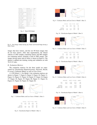
TABLE III
RESULT OF THIRD CNN MODEL
No
Train Validation Test
Loss Accuracy Loss Accuracy Accuracy F1-score
1 0.1171 0.9564 0.2091 0.9242 0.94 0.93
2 0.1627 0.9430 0.2242 0.9015 0.94 0.935
3 0.1342 0.9517 0.2203 0.9318 0.94 0.94
4 0.1772 0.9316 0.2982 0.8864 0.9031 0.905
5 0.1485 0.9416 0.3182 0.8750 0.91 0.91
6 0.1326 0.9484 0.2013 0.9318 0.9354 0.93
7 0.1623 0.9437 0.221 0.9318 0.93 0.93
8 0.1453 0.9437 0.2316 0.9053 0.94 0.935
9 0.1319 0.9504 0.2377 0.8977 0.9161 0.915
10 0.1101 0.9544 0.2105 0.9242 0.9129 0.91
Average 0.1422 0.9465 0.2372 0.911 0.9268 0.924
VI. CONCLUSION AND FUTURE DIRECTIONS
Convolutional Neural Networks are great enough to diag-
nose brain tumors using MRI images. This study resulted
in an accuracy of 94% . The count of convolution layers
affects the quality of classification shown in Figure 67 as more
convolution layers expand the accuracy of results. The process
of image augmentation can develop the alternatives of existing
datasets, thereby raising the classification results.
As this paper is developed by only using CNN, in future,
this paper will be developed by using other hybrid deep
learning algorithm.
Fig. 67. Comparison of Models
REFERENCES
[1] Milica M Badža and Marko Č Barjaktarović. Classification of brain
tumors from mri images using a convolutional neural network. Applied
Sciences, 10(6):1999, 2020.
[2] B Devkota, Abeer Alsadoon, PWC Prasad, AK Singh, and A Elchouemi.
Image segmentation for early stage brain tumor detection using mathemat-
ical morphological reconstruction. Procedia Computer Science, 125:115–
123, 2018.
[3] DC Febrianto, I Soesanti, and HA Nugroho. Convolutional neural network
for brain tumor detection. In IOP Conference Series: Materials Science
and Engineering, volume 771, page 012031. IOP Publishing, 2020.