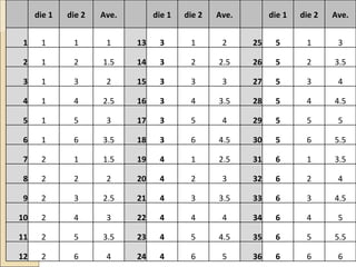
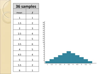
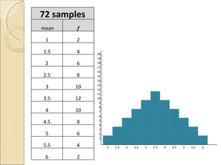
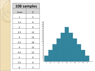
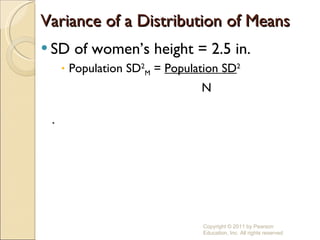
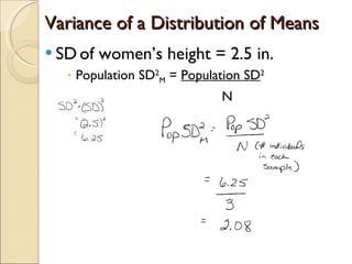
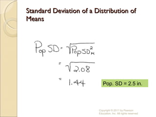
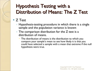
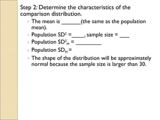
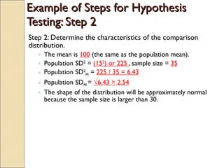
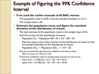
The document discusses distributions of sample means and how they relate to the population from which the samples are drawn. It states that the mean of a distribution of sample means is equal to the population mean. The variance of a distribution of sample means is equal to the population variance divided by the sample size. And the shape of a distribution of sample means approximates a normal distribution if each sample is at least 30 individuals or if the population is normally distributed.

1. Hypothesis Tests with Means of Samples Chapter 6 Copyright © 2011 by Pearson Education, Inc. All rights reserved

2. The Distribution of Means Begin with an example Randomly sample three people from population of women at BAC Compute mean height of sample Population mean = 63.8 in Sample 1 – 67, 66, 62 (ave = 65 in) Sample II – 63, 62, 61 (ave = 62 in) Copyright © 2011 by Pearson Education, Inc. All rights reserved

3. Building a Distribution of Means Think of a distribution of means as if you kept randomly choosing samples of equal sizes from a population and took the means of those samples. Those means are what make up a distribution of means. The characteristics of a distribution of means can be calculated from: characteristics of the population of individuals number of scores in each sample Copyright © 2011 by Pearson Education, Inc. All rights reserved

4. Determining the Characteristics of a Distribution of Means Characteristics of the comparison distribution that you need are: the mean the variance and standard deviation the shape The mean of the distribution of means is about the same as the mean of the original population of individuals. This is true for all distributions of means. The spread of the distribution of means is less than the spread of the distribution of the population of individuals. This is true for all distributions of means. The shape of the distribution of means is approximately normal. This is true for most distributions of means. Copyright © 2011 by Pearson Education, Inc. All rights reserved

5. Mean of a Distribution of Means The mean of a distribution of means of samples of a given size from a particular population It is the same as the mean of the population of individuals. Population M M = Population M Population M M is the mean of the distribution of means. Because the selection process is random and because we are taking a very large number of samples, eventually the high means and the low means perfectly balance each other out. Copyright © 2011 by Pearson Education, Inc. All rights reserved

6. Example 2 Copyright © 2011 by Pearson Education, Inc. All rights reserved

7. die 1 die 2 Ave. die 1 die 2 Ave. die 1 die 2 Ave. 1 1 1 1 13 3 1 2 25 5 1 3 2 1 2 1.5 14 3 2 2.5 26 5 2 3.5 3 1 3 2 15 3 3 3 27 5 3 4 4 1 4 2.5 16 3 4 3.5 28 5 4 4.5 5 1 5 3 17 3 5 4 29 5 5 5 6 1 6 3.5 18 3 6 4.5 30 5 6 5.5 7 2 1 1.5 19 4 1 2.5 31 6 1 3.5 8 2 2 2 20 4 2 3 32 6 2 4 9 2 3 2.5 21 4 3 3.5 33 6 3 4.5 10 2 4 3 22 4 4 4 34 6 4 5 11 2 5 3.5 23 4 5 4.5 35 6 5 5.5 12 2 6 4 24 4 6 5 36 6 6 6

8. 20 19 18 17 16 15 14 13 12 11 10 9 8 7 6 5 4 3 2 1 1 1.5 2 2.5 3 3.5 4 4.5 5 5.5 6 36 samples mean f 1 1 1.5 2 2 3 2.5 4 3 5 3.5 6 4 5 4.5 4 5 3 5.5 2 6 1

9. 20 19 18 17 16 15 14 13 12 11 10 9 8 7 6 5 4 3 2 1 1 1.5 2 2.5 3 3.5 4 4.5 5 5.5 6 72 samples mean f 1 2 1.5 4 2 6 2.5 8 3 10 3.5 12 4 10 4.5 8 5 6 5.5 4 6 2

10. 20 19 18 17 16 15 14 13 12 11 10 9 8 7 6 5 4 3 2 1 1 1.5 2 2.5 3 3.5 4 4.5 5 5.5 6 108 samples mean f 1 3 1.5 6 2 9 2.5 12 3 15 3.5 18 4 15 4.5 12 5 9 5.5 6 6 3

11. 48 47 46 45 44 43 42 41 40 39 38 37 36 35 34 33 32 31 30 29 28 27 26 25 24 23 22 21 20 19 18 17 16 15 14 13 12 11 10 9 8 7 6 5 4 3 2 1 1 1.5 2 2.5 3 3.5 4 4.5 5 5.5 6 288 samples mean f 1 8 1.5 16 2 24 2.5 32 3 40 3.5 48 4 40 4.5 32 5 24 5.5 16 6 8

12. The spread of the distribution of means is less than the spread of the distribution of the population of individuals. This is true for all distributions of means. The distribution of a pop. of individuals The distribution of a sample taken from pop. The distribution of means of samples taken from pop.

13. Variance of a Distribution of Means The variance of a distribution of means is the variance of the population of individuals divided by the number of individuals in each sample. Population SD 2 M = Population SD 2 N Population SD 2 M = the variance of the distribution of means Population SD 2 = the variance of the population of individuals N = number of individuals in each sample . Copyright © 2011 by Pearson Education, Inc. All rights reserved

14. Standard Deviation of a Distribution of Means The standard deviation of a distribution of means is the square root of the variance of the distribution of means comparison distribution. Population SD M = √Population SD 2 M Population SD M = standard deviation of the distribution of means Population SD M is also known as the standard error of the mean. tells you how much the means in the distribution of means deviate from the mean of the population Copyright © 2011 by Pearson Education, Inc. All rights reserved

15. Variance of a Distribution of Means SD of women’s height = 2.5 in. Population SD 2 M = Population SD 2 N . Copyright © 2011 by Pearson Education, Inc. All rights reserved

16. Variance of a Distribution of Means SD of women’s height = 2.5 in. Population SD 2 M = Population SD 2 N

17. Standard Deviation of a Distribution of Means Copyright © 2011 by Pearson Education, Inc. All rights reserved Pop. SD = 2.5 in.

18. The Shape of a Distribution of Means The shape of a distribution of means is approximately normal if either: each sample is of 30 or more individuals or the distribution of the population of individuals is normal Regardless of the shape of the distribution of the population of individuals, the distribution of means tends to be unimodal and symmetrical. Middle scores for means are more likely and extreme means are less likely. A distribution of means tends to be symmetrical because lack of symmetry is caused by extremes. Since there are fewer extremes in a distribution of means, there is less asymmetry. Copyright © 2011 by Pearson Education, Inc. All rights reserved

19. What is the distribution if you only throw one die at a time? (hint-think about the probability of getting each number)

20. die 1 f 1 1 1 2 2 1 3 3 1 4 4 1 5 5 1 6 6 1 6 5 4 3 2 1 1 2 3 4 5 6

21. 20 19 18 17 16 15 14 13 12 11 10 9 8 7 6 5 4 3 2 1 1 1.5 2 2.5 3 3.5 4 4.5 5 5.5 6 36 samples mean f 1 1 1.5 2 2 3 2.5 4 3 5 3.5 6 4 5 4.5 4 5 3 5.5 2 6 1

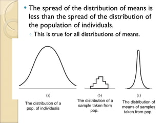
22. Review of the Three Kinds of Distributions Population’s Distribution made up of scores of all individuals in the population could be any shape, but is often normal Population M represents the mean. Population SD 2 represents the variance. Population SD represents the standard deviation. Particular Sample’s Distribution made up of scores of the individuals in a single sample could be any shape M = (∑X) / N calculated from scores of those in the sample SD 2 = [∑(X – M) 2 ] / N SD = √SD 2 Distribution of Means means of samples randomly taken from the population approximately normal if each sample has at least 30 individuals or if population is normal Copyright © 2011 by Pearson Education, Inc. All rights reserved

23. Hypothesis Testing with a Distribution of Means: The Z Test Z Test Hypothesis-testing procedure in which there is a single sample and the population variance is known The comparison distribution for the Z test is a distribution of means. The distribution of means is the distribution to which you compare your sample’s mean to see how likely it is that you could have selected a sample with a mean that extreme if the null hypothesis were true. Copyright © 2011 by Pearson Education, Inc. All rights reserved

24. Figuring the Z Score of a Sample’s Mean on the Distribution of Means If you had a sample with a mean of 25, a distribution of means with a mean of 15, and a standard deviation of 5, the Z score of the sample’s mean would be 2. Z = (M - Population M M ) Population SD M Z = (25 – 15) = 2 5 Copyright © 2011 by Pearson Education, Inc. All rights reserved

25. Figuring the Z Score of a Sample’s Mean on the Distribution of Means Pop. M M = Pop. M mean height = 63.8 Pop. SD = .32 Sample 1 mean = 65 Sample size = 60 Copyright © 2011 by Pearson Education, Inc. All rights reserved

26. Figuring the Z Score of a Sample’s Mean on the Distribution of Means Pop. M M = Pop. M mean height = 63.8 Pop. SD = 1.44 Sample 1 mean = 65

27. Steps for Hypothesis Testing The steps for hypothesis testing are the same for a sample of more than 1 as they are for a sample of 1. Step 1: Restate the question as a research hypothesis and a null hypothesis about the population. Step 2: Determine the characteristics of the comparison distribution. Step 3: Determine the cutoff sample score on the comparison distribution at which the null hypothesis should be rejected. Step 4: Determine your sample’s score on the comparison distribution. Step 5: Decide whether to reject the null hypothesis. Copyright © 2011 by Pearson Education, Inc. All rights reserved

28. Example of Steps for Hypothesis Testing: Step 1 Step 1: Restate the question as a research hypothesis and a null hypothesis about the population. Population 1: Women at BAC Population 2: Women in general H a = Women at BAC are not equal in height to women in general H 0 = Women at BAC are equal in height to women in general

29. Example of Steps for Hypothesis Testing: Step 2 Step 2: Determine the characteristics of the comparison distribution. The comparison distribution is a distribution of means of samples of 60 individuals each. The mean is ______(the same as the population mean). Population SD 2 =____, sample size = ___ Population SD 2 M = ________ Population SD M = The shape of the distribution will be approximately normal because the sample size is larger than 30.

30. Example of Steps for Hypothesis Testing: Step 2 Step 2: Determine the characteristics of the comparison distribution. The comparison distribution is a distribution of means of samples of 60 individuals each. The mean is 63.8 in. (the same as the population mean). Population SD 2 = (2.5 2 ) 6.25 , sample size = 60 Population SD 2 M = 6.25 / 60 = .10 Population SD M = √ .10 = .32 The shape of the distribution will be approximately normal because the sample size is larger than 30.

31. Example of Steps for Hypothesis Testing: Step 3 Step 3: Determine the cutoff sample score on the comparison distribution at which the null hypothesis should be rejected. Significance level p<.05 One-tailed or Two-Tailed? What is the cutoff Z?

32. Example of Steps for Hypothesis Testing: Step 3 Step 3: Determine the cutoff sample score on the comparison distribution at which the null hypothesis should be rejected. Significance level p<.05 Two-Tailed Cutoff Z = -1.96 & +1.96

33. Example of Steps for Hypothesis Testing: Step 4 Step 4: Determine your sample’s score on the comparison distribution. Sample 1 mean = 65 in.

34. Example of Steps for Hypothesis Testing: Step 5 Step 5: Decide whether to reject the null hypothesis. Z =3.75

35. Example of Steps for Hypothesis Testing: Step 5 Step 5: Decide whether to reject the null hypothesis. Reject the null hypothesis Find support for the research hypothesis that BAC women’s height is not equal to women in general

36. Steps for Hypothesis Testing The steps for hypothesis testing are the same for a sample of more than 1 as they are for a sample of 1. Step 1: Restate the question as a research hypothesis and a null hypothesis about the population. Step 2: Determine the characteristics of the comparison distribution. Step 3: Determine the cutoff sample score on the comparison distribution at which the null hypothesis should be rejected. Step 4: Determine your sample’s score on the comparison distribution. Step 5: Decide whether to reject the null hypothesis. Copyright © 2011 by Pearson Education, Inc. All rights reserved

37. After-school example H a = Children in academic after-school programs will have higher IQ scores than children in the general population. H 0 = Children in academic after-school programs will not have higher IQ scores than children in the general population. Population mean = 100 Population SD = 15 Sample mean = 107 Sample size = 35 children Copyright © 2011 by Pearson Education, Inc. All rights reserved

38. Step 1: Restate the question as a research hypothesis and a null hypothesis about the population. Population 1: Children who participate in academic after-school program Population 2: Children in general H a = Children in academic after-school programs will have higher IQ scores than children in the general population. H 0 = Children in academic after-school programs will not have higher IQ scores than children in the general population.

39. Step 2: Determine the characteristics of the comparison distribution. The mean is ______(the same as the population mean). Population SD 2 =____, sample size = ___ Population SD 2 M = ________ Population SD M = The shape of the distribution will be approximately normal because the sample size is larger than 30.

40. Example of Steps for Hypothesis Testing: Step 2 Step 2: Determine the characteristics of the comparison distribution. The mean is 100 (the same as the population mean). Population SD 2 = (15 2 ) or 225 , sample size = 35 Population SD 2 M = 225 / 35 = 6.43 Population SD M = √ 6.43 = 2.54 The shape of the distribution will be approximately normal because the sample size is larger than 30.

41. Example of Steps for Hypothesis Testing: Step 3 Step 3: Determine the cutoff sample score on the comparison distribution at which the null hypothesis should be rejected. Significance level p<.01 One-tailed or Two-Tailed? What is the cutoff Z?

42. Example of Steps for Hypothesis Testing: Step 3 Step 3: Determine the cutoff sample score on the comparison distribution at which the null hypothesis should be rejected. Significance level p<.01 One-Tailed Cutoff Z = +2.32

43. Example of Steps for Hypothesis Testing: Step 4 Step 4: Determine your sample’s score on the comparison distribution. Sample 1 mean = 107

44. Example of Steps for Hypothesis Testing: Step 5 Step 5: Decide whether to reject the null hypothesis.

45. Example of Steps for Hypothesis Testing: Step 5 Step 5: Decide whether to reject the null hypothesis. A mean of 107 is 2.76 standard deviations above the mean of the distribution of means Reject the null hypothesis (support the research hypothesis) Children who attend academic after-school programs have higher IQ scores than children who do not attend the programs.

46. Hypothesis Tests about Means of Samples in Research Articles Z tests are not often seen in research articles because it is rare to know a population’s mean and standard deviation. Copyright © 2011 by Pearson Education, Inc. All rights reserved

47. Advanced Topic: Estimation and Confidence Intervals Estimating the population mean based on the scores in a sample is an important approach in experimental and survey research. When the population mean is unknown, the best estimate of the population mean is the sample mean. The accuracy of the population mean estimate is the standard deviation of the distribution of means (standard error). Copyright © 2011 by Pearson Education, Inc. All rights reserved

48. Range of Possible Means Likely to Include the Population Mean Confidence Interval used to get a sense of the accuracy of an estimated population mean It is the range of population means from which it is not highly unlikely that you could have obtained your sample mean. 95% confidence interval confidence interval for which there is approximately a 95% change that the population mean falls in this interval Z scores from -1.96 to +1.96 on the distribution of means 99% confidence interval confidence interval for which there is approximately a 99% chance that the population mean falls in this interval Z scores from -2.58 to +2.58 confidence limit upper and lower value of a confidence interval Copyright © 2011 by Pearson Education, Inc. All rights reserved

49. Figuring the 95% and 99% Confidence Intervals Estimate the population mean and figure the standard deviation of the distribution of means. The best estimate of the population mean is the sample mean. Find the variance of the distribution of means. Population S 2 M = Population SD 2 / N Take the square root of the variance of the distribution of means to find the standard deviation of the distribution of means. Population SD M = √Population SD 2 M Find the Z scores that go with the confidence interval you want. 95% CI Z scores are +1.96 and -1.96 99% CI Z scores are +2.58 and -2.58 To find the confidence interval, change these Z scores to raw scores . Copyright © 2011 by Pearson Education, Inc. All rights reserved

50. Example of Figuring the 99% Confidence Interval If we used the earlier example of 60 BAC women The population mean is 63.8 in and the standard deviation is 2.5 in. The sample mean is 65. Estimate the population mean and figure the standard deviation of the distribution of means. The best estimate of the population mean is the sample mean of 65. Find the variance of the distribution of means. Population S 2 M = Population SD 2 / N = 2.5 2 / 60= .10 Take the square root of the variance of the distribution of means to find the standard deviation of the distribution of means. Population SD M = √Population SD 2 M = √.10 = .32 Find the Z scores that go with the confidence interval you want . 99% CI Z scores are +2.58 and -2.58 To find the confidence interval ,change these Z scores to raw scores. lower limit = (-2.58)(.32) + 65 = -.83 + 65 = 64.17 upper limit = (+2.58)(.32) + 65 = .83 + 65 = 65.83

51. Example of Figuring the 95% Confidence Interval If we used the earlier example of 35 children who participated in academic after-school program The population mean is 100 and the standard deviation is 15 The sample mean is 107. Estimate the population mean and figure the standard deviation of the distribution of means. The best estimate of the population mean is the sample mean of 107. Find the variance of the distribution of means. Population S 2 M = Population SD 2 / N = 15 2 / 35= 6.43 Take the square root of the variance of the distribution of means to find the standard deviation of the distribution of means. Population SD M = √Population SD 2 M = √6.43=2.54 Find the Z scores that go with the confidence interval you want . 99% CI Z scores are +1.96 and -1.96 To find the confidence interval ,change these Z scores to raw scores. lower limit = (-1.96)(2.54.) + 107 = -.4.98 + 107 = 102.02 upper limit = (+1.96)(2.54) + 107 = .4.98 + 107 = 111.98

52. Confidence Intervals In Research Articles Confidence intervals are becoming more common in research articles in some fields. Copyright © 2011 by Pearson Education, Inc. All rights reserved