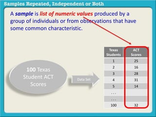
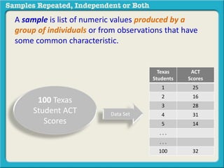
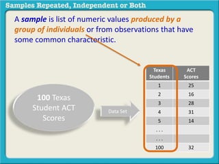
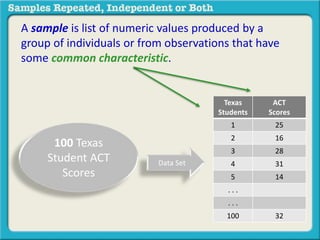
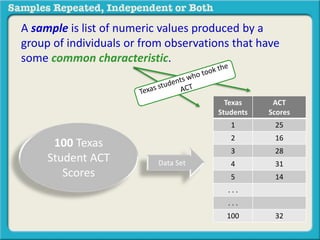
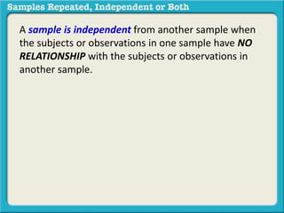
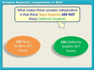
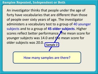
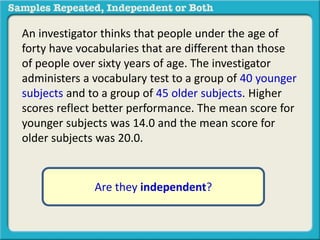
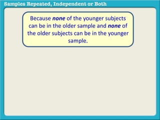
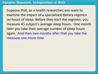
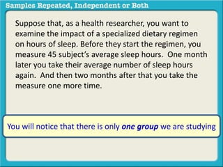
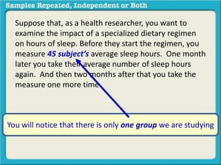
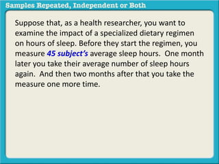
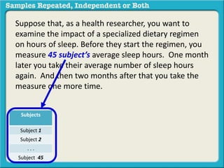
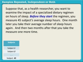
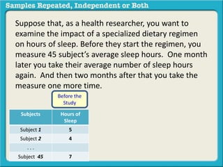
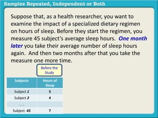
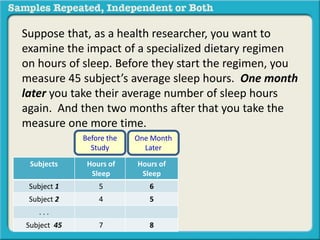
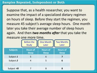
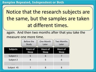
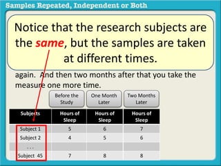
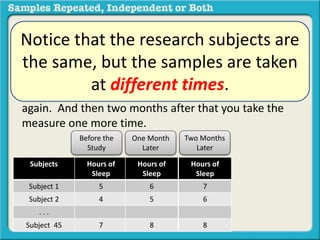
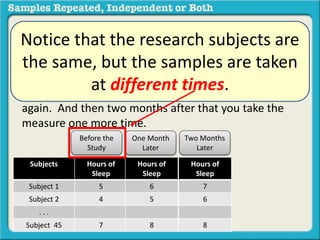
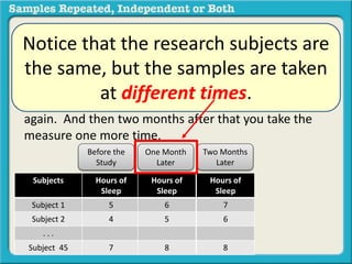
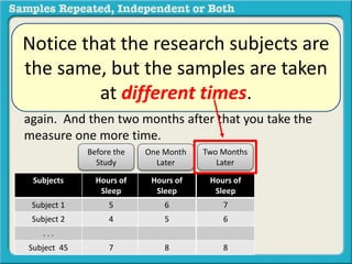
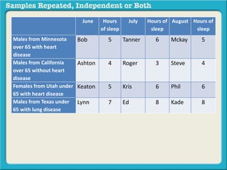
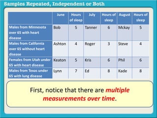
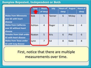
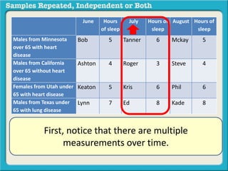
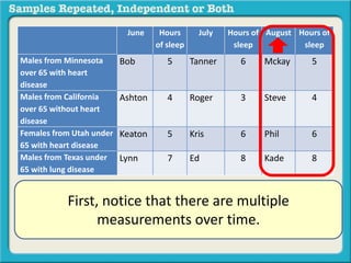
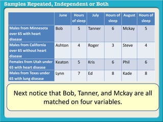
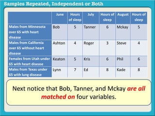
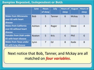
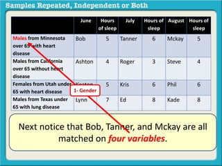
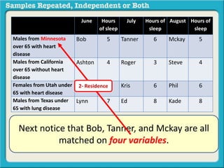
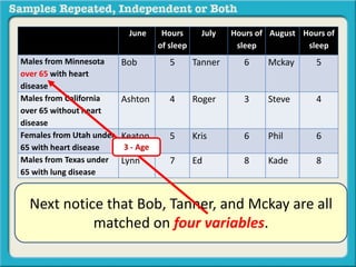
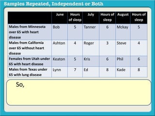
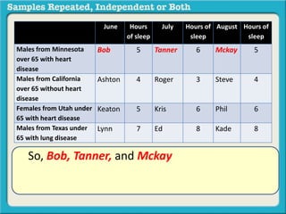
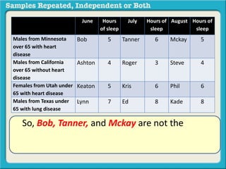
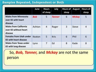
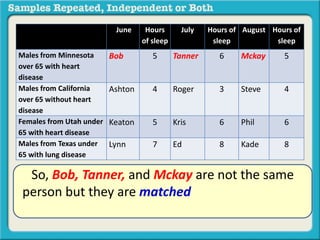
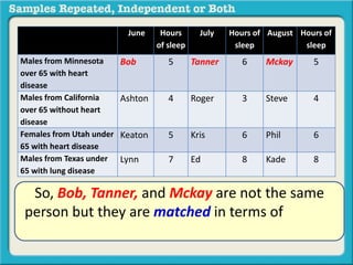
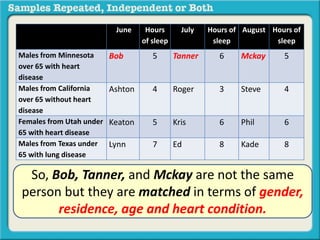
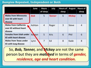
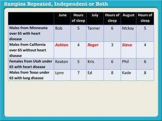
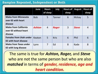
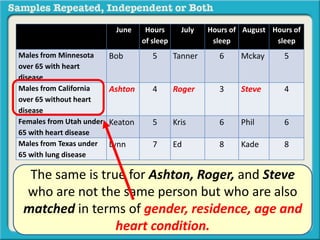
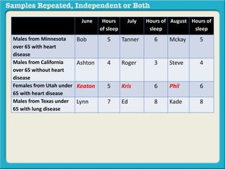
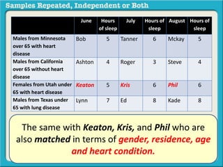
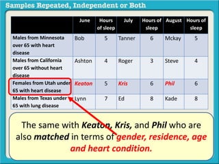
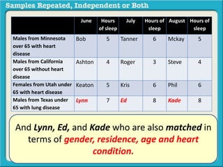
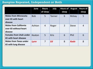
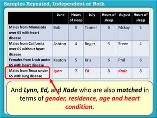
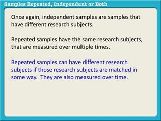
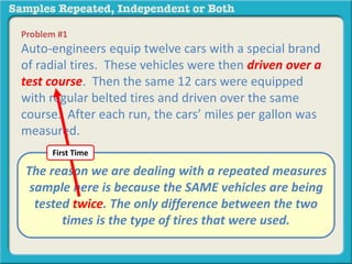
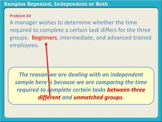
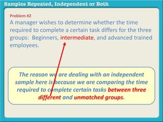
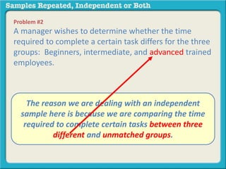
The document discusses independent and repeated samples. An independent sample involves subjects or observations from one sample that have no relationship with subjects or observations from another sample. A repeated sample involves measuring the same subjects or matched subjects more than once. An example is given of a study measuring sleep hours in the same subjects before and after starting a dietary regimen to examine the impact of the regimen over time. This uses a repeated sample as the same subjects are measured on multiple occasions.

1. You will now determine if the samples you are working
with are independent or repeated.

2. Your options will be:

3. Your options will be:
Independent Samples
Repeated Samples

4. What is a sample?

5. A sample is list of numeric values produced by a group
of individuals or from observations that have some
common characteristic.

6. What does this mean?

7. Let’s look at an example:

8. You have been asked to determine if ACT scores from
Texas students are similar to national student ACT scores.

9. You have been asked to determine if ACT scores from
Texas students are similar to national student ACT scores.
You select a sample of 100 student ACT scores from Texas
and determine if they are statistically similar to national
ACT scores.

10. Let’s go back to our definition of a sample:

11. A sample is list of numeric values produced by a group
of individuals or from observations that have some
common characteristic.

12. Here is the problem again:

13. Here is the problem again:
You have been asked to determine if ACT scores from
Texas students are similar to national student ACT
scores. You select a sample of 100 student ACT scores
from Texas and determine if they are statistically similar
to national ACT scores.

14. Here is the problem again:
You have been asked to determine if ACT scores from
Texas students are similar to national student ACT
scores. You select a sample of 100 student ACT scores
from Texas and determine if they are statistically similar
to national ACT scores.
What are the numeric values in this problem?

15. Here is the problem again:
You have been asked to determine if ACT scores from
Texas students are similar to national student ACT
scores. You select a sample of 100 student ACT scores
from Texas and determine if they are statistically similar
to national ACT scores.
What are the numeric values in this problem?
ACT scores

16. Here is the problem again:
You have been asked to determine if ACT scores from
Texas students are similar to national student ACT
scores. You select a sample of 100 student ACT scores
from Texas and determine if they are statistically similar
to national ACT scores.
What group produced these scores?

17. Here is the problem again:
You have been asked to determine if ACT scores from
Texas students are similar to national student ACT
scores. You select a sample of 100 student ACT scores
from Texas and determine if they are statistically similar
to national ACT scores.
What group produced these scores?
Texas Students

18. Here is the problem again:
You have been asked to determine if ACT scores from
Texas students are similar to national student ACT
scores. You select a sample of 100 student ACT scores
from Texas and determine if they are statistically similar
to national ACT scores.
What is the basis for group membership?

19. Here is the problem again:
You have been asked to determine if ACT scores from
Texas students are similar to national student ACT
scores. You select a sample of 100 student ACT scores
from Texas and determine if they are statistically similar
to national ACT scores.
What is the basis for group membership?
Being a student from Texas who took the ACT

20. Here is what that sample might look like:

21. Here is what that sample might look like:
100 Texas
Student ACT
Scores

22. Here is what that sample might look like:
100 Texas
Student ACT
Scores
Data Set

23. Here is what that sample might look like:
100 Texas
Student ACT
Scores
Texas
Students
ACT
Scores
1 25
2 16
3 28
4 31
5 14
. . .
. . .
100 32
Data Set

24. 100 Texas
Student ACT
Scores
Texas
Students
ACT
Scores
1 25
2 16
3 28
4 31
5 14
. . .
. . .
100 32
Data Set
Back to the definition:

25. A sample is list of numeric values produced by a
group of individuals or from observations that have
some common characteristic.
100 Texas
Student ACT
Scores
Texas
Students
ACT
Scores
1 25
2 16
3 28
4 31
5 14
. . .
. . .
100 32
Data Set

26. A sample is list of numeric values produced by a
group of individuals or from observations that have
some common characteristic.
100 Texas
Student ACT
Scores
Texas
Students
ACT
Scores
1 25
2 16
3 28
4 31
5 14
. . .
. . .
100 32
Data Set

27. A sample is list of numeric values produced by a
group of individuals or from observations that have
some common characteristic.
100 Texas
Student ACT
Scores
Texas
Students
ACT
Scores
1 25
2 16
3 28
4 31
5 14
. . .
. . .
100 32
Data Set

28. A sample is list of numeric values produced by a
group of individuals or from observations that have
some common characteristic.
100 Texas
Student ACT
Scores
Texas
Students
ACT
Scores
1 25
2 16
3 28
4 31
5 14
. . .
. . .
100 32
Data Set

29. A sample is list of numeric values produced by a
group of individuals or from observations that have
some common characteristic.
100 Texas
Student ACT
Scores
Texas
Students
ACT
Scores
1 25
2 16
3 28
4 31
5 14
. . .
. . .
100 32
Data Set

30. A sample is list of numeric values produced by a
group of individuals or from observations that have
some common characteristic.
100 Texas
Student ACT
Scores
Texas
Students
ACT
Scores
1 25
2 16
3 28
4 31
5 14
. . .
. . .
100 32
Data Set

31. Now that you’ve been introduced to what sample is

32. Now that you’ve been introduced to what sample is
. . . What are Independent Samples?

33. A sample is independent from another sample when
the subjects or observations in one sample have NO
RELATIONSHIP with the subjects or observations in
another sample.

34. For example:

35. Imagine you have been asked to compare ACT scores
between Texas and California students.

36. What makes these samples independent
is that these Texas Students ARE NOT
these California Students

37. What makes these samples independent
is that these Texas Students ARE NOT
these California Students
100 Texas
Student ACT
Scores

38. What makes these samples independent
is that these Texas Students ARE NOT
these California Students
100 Texas
Student ACT
Scores

39. What makes these samples independent
is that these Texas Students ARE NOT
these California Students
100 Texas
Student ACT
Scores
100 California
Student ACT
Scores

40. This may seem very obvious that one groups
individuals are not the other groups individuals.

41. This may seem very obvious that one groups
individuals are not the other groups individuals. But,
it is an important aspect that makes independent
samples – independent!

42. Consider the following example:

43. An investigator thinks that people under the age of
forty have vocabularies that are different than those
of people over sixty years of age. The investigator
administers a vocabulary test to a group of 40 younger
subjects and to a group of 45 older subjects. Higher
scores reflect better performance. The mean score for
younger subjects was 14.0 and the mean score for
older subjects was 20.0.

44. An investigator thinks that people under the age of
forty have vocabularies that are different than those
of people over sixty years of age. The investigator
administers a vocabulary test to a group of 40 younger
subjects and to a group of 45 older subjects. Higher
scores reflect better performance. The mean score for
younger subjects was 14.0 and the mean score for
older subjects was 20.0.

45. An investigator thinks that people under the age of
forty have vocabularies that are different than those
of people over sixty years of age. The investigator
administers a vocabulary test to a group of 40 younger
subjects and to a group of 45 older subjects. Higher
scores reflect better performance. The mean score for
younger subjects was 14.0 and the mean score for
older subjects was 20.0.

46. An investigator thinks that people under the age of
forty have vocabularies that are different than those
of people over sixty years of age. The investigator
administers a vocabulary test to a group of 40 younger
subjects and to a group of 45 older subjects. Higher
scores reflect better performance. The mean score for
younger subjects was 14.0 and the mean score for
older subjects was 20.0.
How many samples are there?

47. An investigator thinks that people under the age of
forty have vocabularies that are different than those
of people over sixty years of age. The investigator
administers a vocabulary test to a group of 40 younger
subjects and to a group of 45 older subjects. Higher
scores reflect better performance. The mean score for
younger subjects was 14.0 and the mean score for
older subjects was 20.0.
Sample 1
How many samples are there?

48. An investigator thinks that people under the age of
forty have vocabularies that are different than those
of people over sixty years of age. The investigator
administers a vocabulary test to a group of 40 younger
subjects and to a group of 45 older subjects. Higher
scores reflect better performance. The mean score for
younger subjects was 14.0 and the mean score for
older subjects was 20.0.
Sample 2
How many samples are there?

49. An investigator thinks that people under the age of
forty have vocabularies that are different than those
of people over sixty years of age. The investigator
administers a vocabulary test to a group of 40 younger
subjects and to a group of 45 older subjects. Higher
scores reflect better performance. The mean score for
younger subjects was 14.0 and the mean score for
older subjects was 20.0.
Are they independent?

50. Yes, they are independent!

51. Because none of the younger subjects
can be in the older sample and none of
the older subjects can be in the younger
sample.

52. Next:

53. What are repeated samples?

54. With repeated samples the two samples share one
important thing in common:

55. With repeated samples the two samples share one
important thing in common: They are the SAME
PERSONS being measured . . .

56. With repeated samples the two samples share one
important thing in common: They are the SAME
PERSONS being measured more than once . . .

57. With repeated samples the two samples share one
important thing in common: They are the SAME
PERSONS being measured more than once or they are
different persons but MATCHED in some way.

58. Consider this example:

59. Suppose that, as a health researcher, you want to
examine the impact of a specialized dietary regimen
on hours of sleep.

60. Suppose that, as a health researcher, you want to
examine the impact of a specialized dietary regimen
on hours of sleep. Before they start the regimen, you
measure 45 subject’s average sleep hours.

61. Suppose that, as a health researcher, you want to
examine the impact of a specialized dietary regimen
on hours of sleep. Before they start the regimen, you
measure 45 subject’s average sleep hours. One month
later you take their average number of sleep hours
again.

62. Suppose that, as a health researcher, you want to
examine the impact of a specialized dietary regimen
on hours of sleep. Before they start the regimen, you
measure 45 subject’s average sleep hours. One month
later you take their average number of sleep hours
again. And then two months after that you take the
measure one more time.

63. Suppose that, as a health researcher, you want to
examine the impact of a specialized dietary regimen
on hours of sleep. Before they start the regimen, you
measure 45 subject’s average sleep hours. One month
later you take their average number of sleep hours
again. And then two months after that you take the
measure one more time.
You will notice that there is only one group we are studying

64. Suppose that, as a health researcher, you want to
examine the impact of a specialized dietary regimen
on hours of sleep. Before they start the regimen, you
measure 45 subject’s average sleep hours. One month
later you take their average number of sleep hours
again. And then two months after that you take the
measure one more time.
You will notice that there is only one group we are studying

65. Suppose that, as a health researcher, you want to
examine the impact of a specialized dietary regimen
on hours of sleep. Before they start the regimen, you
measure 45 subject’s average sleep hours. One month
later you take their average number of sleep hours
again. And then two months after that you take the
measure one more time.

66. Suppose that, as a health researcher, you want to
examine the impact of a specialized dietary regimen
on hours of sleep. Before they start the regimen, you
measure 45 subject’s average sleep hours. One month
later you take their average number of sleep hours
again. And then two months after that you take the
measure one more time.
Subjects
Subject 1
Subject 2
. . .
Subject 45

67. Suppose that, as a health researcher, you want to
examine the impact of a specialized dietary regimen
on hours of sleep. Before they start the regimen, you
measure 45 subject’s average sleep hours. One month
later you take their average number of sleep hours
again. And then two months after that you take the
measure one more time.
Subjects
Subject 1
Subject 2
. . .
Subject 45

68. Suppose that, as a health researcher, you want to
examine the impact of a specialized dietary regimen
on hours of sleep. Before they start the regimen, you
measure 45 subject’s average sleep hours. One month
later you take their average number of sleep hours
again. And then two months after that you take the
measure one more time.
Before the
Study
Subjects
Subject 1
Subject 2
. . .
Subject 45

69. Suppose that, as a health researcher, you want to
examine the impact of a specialized dietary regimen
on hours of sleep. Before they start the regimen, you
measure 45 subject’s average sleep hours. One month
later you take their average number of sleep hours
again. And then two months after that you take the
measure one more time.
Before the
Study
Subjects Hours of
Sleep
Subject 1 5
Subject 2 4
. . .
Subject 45 7

70. Suppose that, as a health researcher, you want to
examine the impact of a specialized dietary regimen
on hours of sleep. Before they start the regimen, you
measure 45 subject’s average sleep hours. One month
later you take their average number of sleep hours
again. And then two months after that you take the
measure one more time.
Before the
Study
Subjects Hours of
Sleep
Subject 1 5
Subject 2 4
. . .
Subject 45 7

71. Suppose that, as a health researcher, you want to
examine the impact of a specialized dietary regimen
on hours of sleep. Before they start the regimen, you
measure 45 subject’s average sleep hours. One month
later you take their average number of sleep hours
again. And then two months after that you take the
measure one more time.
Before the
Study
Subjects Hours of
Sleep
Subject 1 5
Subject 2 4
. . .
Subject 45 7
One Month
Later
Hours of
Sleep
6
5
8

72. Suppose that, as a health researcher, you want to
examine the impact of a specialized dietary regimen
on hours of sleep. Before they start the regimen, you
measure 45 subject’s average sleep hours. One month
later you take their average number of sleep hours
again. And then two months after that you take the
measure one more time.
Before the
Study
Subjects Hours of
Sleep
Subject 1 5
Subject 2 4
. . .
Subject 45 7
One Month
Later
Hours of
Sleep
6
5
8

73. Suppose that, as a health researcher, you want to
examine the impact of a specialized dietary regimen
on hours of sleep. Before they start the regimen, you
measure 45 subject’s average sleep hours. One month
later you take their average number of sleep hours
again. And then two months after that you take the
measure one more time.
Before the
Study
Subjects Hours of
Hours of Sleep
6
5
8
Sleep
Subject 1 5
Subject 2 4
. . .
Subject 45 7
One Month
Later
Hours of
Sleep
6
5
8
Two Months
Later
Hours of
Sleep
7
6
8

74. Suppose that, as a health researcher, you want to
examine the impact of a specialized dietary regimen
on hours of sleep. Before they start the regimen, you
measure 45 subject’s average sleep hours. One month
later you take their average number of sleep hours
again. And then two months after that you take the
measure one more time.
Notice that the research subjects are
the same, but the samples are taken
at different times.
Before the
Study
Subjects Hours of
Hours of Sleep
6
5
8
Sleep
Subject 1 5
Subject 2 4
. . .
Subject 45 7
One Month
Later
Hours of
Sleep
6
5
8
Two Months
Later
Hours of
Sleep
7
6
8

75. Suppose that, as a health researcher, you want to
examine the impact of a specialized dietary regimen
on hours of sleep. Before they start the regimen, you
measure 45 subject’s average sleep hours. One month
later you take their average number of sleep hours
again. And then two months after that you take the
measure one more time.
Notice that the research subjects are
the same, but the samples are taken
at different times.
Before the
Study
Subjects Hours of
Hours of Sleep
6
5
8
Sleep
Subject 1 5
Subject 2 4
. . .
Subject 45 7
One Month
Later
Hours of
Sleep
6
5
8
Two Months
Later
Hours of
Sleep
7
6
8

76. Suppose that, as a health researcher, you want to
examine the impact of a specialized dietary regimen
on hours of sleep. Before they start the regimen, you
measure 45 subject’s average sleep hours. One month
later you take their average number of sleep hours
again. And then two months after that you take the
measure one more time.
Notice that the research subjects are
the same, but the samples are taken
at different times.
Before the
Study
Subjects Hours of
Hours of Sleep
6
5
8
Sleep
Subject 1 5
Subject 2 4
. . .
Subject 45 7
One Month
Later
Hours of
Sleep
6
5
8
Two Months
Later
Hours of
Sleep
7
6
8

77. Suppose that, as a health researcher, you want to
examine the impact of a specialized dietary regimen
on hours of sleep. Before they start the regimen, you
measure 45 subject’s average sleep hours. One month
later you take their average number of sleep hours
again. And then two months after that you take the
measure one more time.
Notice that the research subjects are
the same, but the samples are taken
at different times.
Before the
Study
Subjects Hours of
Hours of Sleep
6
5
8
Sleep
Subject 1 5
Subject 2 4
. . .
Subject 45 7
One Month
Later
Hours of
Sleep
6
5
8
Two Months
Later
Hours of
Sleep
7
6
8

78. Suppose that, as a health researcher, you want to
examine the impact of a specialized dietary regimen
on hours of sleep. Before they start the regimen, you
measure 45 subject’s average sleep hours. One month
later you take their average number of sleep hours
again. And then two months after that you take the
measure one more time.
Notice that the research subjects are
the same, but the samples are taken
at different times.
Before the
Study
Subjects Hours of
Hours of Sleep
6
5
8
Sleep
Subject 1 5
Subject 2 4
. . .
Subject 45 7
One Month
Later
Hours of
Sleep
6
5
8
Two Months
Later
Hours of
Sleep
7
6
8

79. Suppose that, as a health researcher, you want to
examine the impact of a specialized dietary regimen
on hours of sleep. Before they start the regimen, you
measure 45 subject’s average sleep hours. One month
later you take their average number of sleep hours
again. And then two months after that you take the
measure one more time.
Notice that the research subjects are
the same, but the samples are taken
at different times.
Before the
Study
Subjects Hours of
Hours of Sleep
6
5
8
Sleep
Subject 1 5
Subject 2 4
. . .
Subject 45 7
One Month
Later
Hours of
Sleep
6
5
8
Two Months
Later
Hours of
Sleep
7
6
8

80. These samples are repeated because in this case each
sample has the same person in it being measured
repeatedly.

81. In some instances, the persons are not the same but
are matched on some variable.

82. In some instances, the persons are not the same but
are matched on some variable.
In such a scenario, the samples would be considered
to be repeated.

83. Consider the next example:

84. June Hours
of sleep
July Hours of
sleep
August Hours of
sleep
Males from Minnesota
over 65 with heart
disease
Bob 5 Tanner 6 Mckay 5
Males from California
over 65 without heart
disease
Ashton 4 Roger 3 Steve 4
Females from Utah under
65 with heart disease
Keaton 5 Kris 6 Phil 6
Males from Texas under
65 with lung disease
Lynn 7 Ed 8 Kade 8

85. June Hours
of sleep
July Hours of
sleep
August Hours of
sleep
Males from Minnesota
over 65 with heart
disease
Bob 5 Tanner 6 Mckay 5
Males from California
over 65 without heart
disease
Ashton 4 Roger 3 Steve 4
Females from Utah under
65 with heart disease
Keaton 5 Kris 6 Phil 6
Males from Texas under
65 with lung disease
Lynn 7 Ed 8 Kade 8
First, notice that there are multiple
measurements over time.

86. June Hours
of sleep
July Hours of
sleep
August Hours of
sleep
Males from Minnesota
over 65 with heart
disease
Bob 5 Tanner 6 Mckay 5
Males from California
over 65 without heart
disease
Ashton 4 Roger 3 Steve 4
Females from Utah under
65 with heart disease
Keaton 5 Kris 6 Phil 6
Males from Texas under
65 with lung disease
Lynn 7 Ed 8 Kade 8
First, notice that there are multiple
measurements over time.

87. June Hours
of sleep
July Hours of
sleep
August Hours of
sleep
Males from Minnesota
over 65 with heart
disease
Bob 5 Tanner 6 Mckay 5
Males from California
over 65 without heart
disease
Ashton 4 Roger 3 Steve 4
Females from Utah under
65 with heart disease
Keaton 5 Kris 6 Phil 6
Males from Texas under
65 with lung disease
Lynn 7 Ed 8 Kade 8
First, notice that there are multiple
measurements over time.

88. June Hours
of sleep
July Hours of
sleep
August Hours of
sleep
Males from Minnesota
over 65 with heart
disease
Bob 5 Tanner 6 Mckay 5
Males from California
over 65 without heart
disease
Ashton 4 Roger 3 Steve 4
Females from Utah under
65 with heart disease
Keaton 5 Kris 6 Phil 6
Males from Texas under
65 with lung disease
Lynn 7 Ed 8 Kade 8
First, notice that there are multiple
measurements over time.

89. June Hours
of sleep
July Hours of
sleep
August Hours of
sleep
Males from Minnesota
over 65 with heart
disease
Bob 5 Tanner 6 Mckay 5
Males from California
over 65 without heart
disease
Ashton 4 Roger 3 Steve 4
Females from Utah under
65 with heart disease
Keaton 5 Kris 6 Phil 6
Males from Texas under
65 with lung disease
Lynn 7 Ed 8 Kade 8
Next notice that Bob, Tanner, and Mckay are all
matched on four variables.

90. June Hours
of sleep
July Hours of
sleep
August Hours of
sleep
Males from Minnesota
over 65 with heart
disease
Bob 5 Tanner 6 Mckay 5
Males from California
over 65 without heart
disease
Ashton 4 Roger 3 Steve 4
Females from Utah under
65 with heart disease
Keaton 5 Kris 6 Phil 6
Males from Texas under
65 with lung disease
Lynn 7 Ed 8 Kade 8
Next notice that Bob, Tanner, and Mckay are all
matched on four variables.

91. June Hours
of sleep
July Hours of
sleep
August Hours of
sleep
Males from Minnesota
over 65 with heart
disease
Bob 5 Tanner 6 Mckay 5
Males from California
over 65 without heart
disease
Ashton 4 Roger 3 Steve 4
Females from Utah under
65 with heart disease
Keaton 5 Kris 6 Phil 6
Males from Texas under
65 with lung disease
Lynn 7 Ed 8 Kade 8
Next notice that Bob, Tanner, and Mckay are all
matched on four variables.

92. June Hours
of sleep
July Hours of
sleep
August Hours of
sleep
Males from Minnesota
over 65 with heart
disease
Bob 5 Tanner 6 Mckay 5
Males from California
over 65 without heart
disease
Ashton 4 Roger 3 Steve 4
Females from Utah under
65 with heart disease
Keaton 5 Kris 6 Phil 6
Males from Texas under
65 with lung disease
Lynn 7 Ed 8 Kade 8
Next notice that Bob, Tanner, and Mckay are all
matched on four variables.

93. June Hours
of sleep
July Hours of
sleep
August Hours of
sleep
Males from Minnesota
over 65 with heart
disease
Bob 5 Tanner 6 Mckay 5
Males from California
over 65 without heart
disease
Ashton 4 Roger 3 Steve 4
Females from Utah under
65 with heart disease
Keaton 5 Kris 6 Phil 6
Males from Texas under
65 with lung disease
Lynn 7 Ed 8 Kade 8
Next notice that Bob, Tanner, and Mckay are all
matched on four variables.

94. June Hours
of sleep
July Hours of
sleep
August Hours of
sleep
Males from Minnesota
over 65 with heart
disease
Bob 5 Tanner 6 Mckay 5
Males from California
over 65 without heart
disease
Ashton 4 Roger 3 Steve 4
Females from Utah under
65 with heart disease
Keaton 5 Kris 6 Phil 6
Males from Texas under
65 with lung disease
Lynn 7 Ed 8 Kade 8
Next notice that Bob, Tanner, and Mckay are all
matched on four variables.

95. June Hours
of sleep
July Hours of
sleep
August Hours of
sleep
Males from Minnesota
over 65 with heart
disease
Bob 5 Tanner 6 Mckay 5
Males from California
over 65 without heart
disease
Ashton 4 Roger 3 Steve 4
Females from Utah under
65 with heart disease
Keaton 5 Kris 6 Phil 6
Males from Texas under
65 with lung disease
1- Gender
Lynn 7 Ed 8 Kade 8
Next notice that Bob, Tanner, and Mckay are all
matched on four variables.

96. June Hours
of sleep
July Hours of
sleep
August Hours of
sleep
Males from Minnesota
over 65 with heart
disease
Bob 5 Tanner 6 Mckay 5
Males from California
over 65 without heart
disease
Ashton 4 Roger 3 Steve 4
Females from Utah under
65 with heart disease
Keaton 5 Kris 6 Phil 6
Males from Texas under
65 with lung disease
2- Residence
Lynn 7 Ed 8 Kade 8
Next notice that Bob, Tanner, and Mckay are all
matched on four variables.

97. June Hours
of sleep
July Hours of
sleep
August Hours of
sleep
Males from Minnesota
over 65 with heart
disease
Bob 5 Tanner 6 Mckay 5
Males from California
over 65 without heart
disease
Ashton 4 Roger 3 Steve 4
Females from Utah under
65 with heart disease
Keaton 5 Kris 6 Phil 6
Males from Texas under
65 with lung disease
3 - Age
Lynn 7 Ed 8 Kade 8
Next notice that Bob, Tanner, and Mckay are all
matched on four variables.

98. June Hours
of sleep
July Hours of
sleep
August Hours of
sleep
Males from Minnesota
over 65 with heart
disease
Bob 5 Tanner 6 Mckay 5
Males from California
over 65 without heart
disease
Ashton 4 Roger 3 Steve 4
Females from Utah under
65 with heart disease
Keaton 5 Kris 6 Phil 6
Males from Texas under
65 with lung disease
4- Heart
Condition
Lynn 7 Ed 8 Kade 8
Next notice that Bob, Tanner, and Mckay are all
matched on four variables.

99. June Hours
of sleep
July Hours of
sleep
August Hours of
sleep
Males from Minnesota
over 65 with heart
disease
Bob 5 Tanner 6 Mckay 5
Males from California
over 65 without heart
disease
Ashton 4 Roger 3 Steve 4
Females from Utah under
65 with heart disease
Keaton 5 Kris 6 Phil 6
Males from Texas under
65 with lung disease
Lynn 7 Ed 8 Kade 8
So, Bob, Tanner, and Mckay are not the same
person but they are matched in terms of gender,
residence, age and heart condition.

100. June Hours
of sleep
July Hours of
sleep
August Hours of
sleep
Males from Minnesota
over 65 with heart
disease
Bob 5 Tanner 6 Mckay 5
Males from California
over 65 without heart
disease
Ashton 4 Roger 3 Steve 4
Females from Utah under
65 with heart disease
Keaton 5 Kris 6 Phil 6
Males from Texas under
65 with lung disease
Lynn 7 Ed 8 Kade 8
So, Bob, Tanner, and Mckay are not the same
person but they are matched in terms of gender,
residence, age and heart condition.

101. June Hours
of sleep
July Hours of
sleep
August Hours of
sleep
Males from Minnesota
over 65 with heart
disease
Bob 5 Tanner 6 Mckay 5
Males from California
over 65 without heart
disease
Ashton 4 Roger 3 Steve 4
Females from Utah under
65 with heart disease
Keaton 5 Kris 6 Phil 6
Males from Texas under
65 with lung disease
Lynn 7 Ed 8 Kade 8
So, Bob, Tanner, and Mckay are not the same
person but they are matched in terms of gender,
residence, age and heart condition.

102. June Hours
of sleep
July Hours of
sleep
August Hours of
sleep
Males from Minnesota
over 65 with heart
disease
Bob 5 Tanner 6 Mckay 5
Males from California
over 65 without heart
disease
Ashton 4 Roger 3 Steve 4
Females from Utah under
65 with heart disease
Keaton 5 Kris 6 Phil 6
Males from Texas under
65 with lung disease
Lynn 7 Ed 8 Kade 8
So, Bob, Tanner, and Mckay are not the same
person but they are matched in terms of gender,
residence, age and heart condition.

103. June Hours
of sleep
July Hours of
sleep
August Hours of
sleep
Males from Minnesota
over 65 with heart
disease
Bob 5 Tanner 6 Mckay 5
Males from California
over 65 without heart
disease
Ashton 4 Roger 3 Steve 4
Females from Utah under
65 with heart disease
Keaton 5 Kris 6 Phil 6
Males from Texas under
65 with lung disease
Lynn 7 Ed 8 Kade 8
So, Bob, Tanner, and Mckay are not the same
person but they are matched in terms of gender,
residence, age and heart condition.

104. June Hours
of sleep
July Hours of
sleep
August Hours of
sleep
Males from Minnesota
over 65 with heart
disease
Bob 5 Tanner 6 Mckay 5
Males from California
over 65 without heart
disease
Ashton 4 Roger 3 Steve 4
Females from Utah under
65 with heart disease
Keaton 5 Kris 6 Phil 6
Males from Texas under
65 with lung disease
Lynn 7 Ed 8 Kade 8
So, Bob, Tanner, and Mckay are not the same
person but they are matched in terms of gender,
residence, age and heart condition.

105. June Hours
of sleep
July Hours of
sleep
August Hours of
sleep
Males from Minnesota
over 65 with heart
disease
Bob 5 Tanner 6 Mckay 5
Males from California
over 65 without heart
disease
Ashton 4 Roger 3 Steve 4
Females from Utah under
65 with heart disease
Keaton 5 Kris 6 Phil 6
Males from Texas under
65 with lung disease
Lynn 7 Ed 8 Kade 8
So, Bob, Tanner, and Mckay are not the same
person but they are matched in terms of gender,
residence, age and heart condition.

106. June Hours
of sleep
July Hours of
sleep
August Hours of
sleep
Males from Minnesota
over 65 with heart
disease
Bob 5 Tanner 6 Mckay 5
Males from California
over 65 without heart
disease
Ashton 4 Roger 3 Steve 4
Females from Utah under
65 with heart disease
Keaton 5 Kris 6 Phil 6
Males from Texas under
65 with lung disease
Lynn 7 Ed 8 Kade 8
So, Bob, Tanner, and Mckay are not the same
person but they are matched in terms of gender,
residence, age and heart condition.

107. June Hours
of sleep
July Hours of
sleep
August Hours of
sleep
Males from Minnesota
over 65 with heart
disease
Bob 5 Tanner 6 Mckay 5
Males from California
over 65 without heart
disease
Ashton 4 Roger 3 Steve 4
Females from Utah under
65 with heart disease
Keaton 5 Kris 6 Phil 6
Males from Texas under
65 with lung disease
Lynn 7 Ed 8 Kade 8

108. June Hours
of sleep
July Hours of
sleep
August Hours of
sleep
Males from Minnesota
over 65 with heart
disease
Bob 5 Tanner 6 Mckay 5
Males from California
over 65 without heart
disease
Ashton 4 Roger 3 Steve 4
Females from Utah under
65 with heart disease
Keaton 5 Kris 6 Phil 6
Males from Texas under
65 with lung disease
Lynn 7 Ed 8 Kade 8
The same is true for Ashton, Roger, and Steve
who are not the same person but who are also
matched in terms of gender, residence, age and
heart condition.

109. June Hours
of sleep
July Hours of
sleep
August Hours of
sleep
Males from Minnesota
over 65 with heart
disease
Bob 5 Tanner 6 Mckay 5
Males from California
over 65 without heart
disease
Ashton 4 Roger 3 Steve 4
Females from Utah under
65 with heart disease
Keaton 5 Kris 6 Phil 6
Males from Texas under
65 with lung disease
Lynn 7 Ed 8 Kade 8
The same is true for Ashton, Roger, and Steve
who are not the same person but who are also
matched in terms of gender, residence, age and
heart condition.

110. June Hours
of sleep
July Hours of
sleep
August Hours of
sleep
Males from Minnesota
over 65 with heart
disease
Bob 5 Tanner 6 Mckay 5
Males from California
over 65 without heart
disease
Ashton 4 Roger 3 Steve 4
Females from Utah under
65 with heart disease
Keaton 5 Kris 6 Phil 6
Males from Texas under
65 with lung disease
Lynn 7 Ed 8 Kade 8

111. June Hours
of sleep
July Hours of
sleep
August Hours of
sleep
Males from Minnesota
over 65 with heart
disease
Bob 5 Tanner 6 Mckay 5
Males from California
over 65 without heart
disease
Ashton 4 Roger 3 Steve 4
Females from Utah under
65 with heart disease
Keaton 5 Kris 6 Phil 6
Males from Texas under
65 with lung disease
Lynn 7 Ed 8 Kade 8
The same with Keaton, Kris, and Phil who are
also matched in terms of gender, residence, age
and heart condition.

112. June Hours
of sleep
July Hours of
sleep
August Hours of
sleep
Males from Minnesota
over 65 with heart
disease
Bob 5 Tanner 6 Mckay 5
Males from California
over 65 without heart
disease
Ashton 4 Roger 3 Steve 4
Females from Utah under
65 with heart disease
Keaton 5 Kris 6 Phil 6
Males from Texas under
65 with lung disease
Lynn 7 Ed 8 Kade 8
The same with Keaton, Kris, and Phil who are
also matched in terms of gender, residence, age
and heart condition.

113. June Hours
of sleep
July Hours of
sleep
August Hours of
sleep
Males from Minnesota
over 65 with heart
disease
Bob 5 Tanner 6 Mckay 5
Males from California
over 65 without heart
disease
Ashton 4 Roger 3 Steve 4
Females from Utah under
65 with heart disease
Keaton 5 Kris 6 Phil 6
Males from Texas under
65 with lung disease
Lynn 7 Ed 8 Kade 8
And Lynn, Ed, and Kade who are also matched in
terms of gender, residence, age and heart
condition.

114. June Hours
of sleep
July Hours of
sleep
August Hours of
sleep
Males from Minnesota
over 65 with heart
disease
Bob 5 Tanner 6 Mckay 5
Males from California
over 65 without heart
disease
Ashton 4 Roger 3 Steve 4
Females from Utah under
65 with heart disease
Keaton 5 Kris 6 Phil 6
Males from Texas under
65 with lung disease
Lynn 7 Ed 8 Kade 8

115. June Hours
of sleep
July Hours of
sleep
August Hours of
sleep
Males from Minnesota
over 65 with heart
disease
Bob 5 Tanner 6 Mckay 5
Males from California
over 65 without heart
disease
Ashton 4 Roger 3 Steve 4
Females from Utah under
65 with heart disease
Keaton 5 Kris 6 Phil 6
Males from Texas under
65 with lung disease
Lynn 7 Ed 8 Kade 8
And Lynn, Ed, and Kade who are also matched in
terms of gender, residence, age and heart
condition.

116. In summary,

117. In summary,
With repeated samples you are measuring either the
same people over time or the same kind of person
over time (matched)

118. Once again, independent samples are samples that
have different research subjects.

119. Once again, independent samples are samples that
have different research subjects.
Repeated samples have the same research subjects,
that are measured over multiple times.

120. Once again, independent samples are samples that
have different research subjects.
Repeated samples have the same research subjects,
that are measured over multiple times.
Repeated samples can have different research
subjects if those research subjects are matched in
some way. They are also measured over time.

121. In this Guided Practice you will be presented with two
word problems. You will be asked to determine if the
word problem is depicting an independent or repeated
measure samples.

122. Problem #1

123. Problem #1
Auto-engineers equip twelve cars with a special brand
of radial tires. These vehicles were then driven over a
test course. Then the same 12 cars were equipped
with regular belted tires and driven over the same
course. After each run, the cars’ miles per gallon was
measured.

124. Problem #1
Auto-engineers equip twelve cars with a special brand
of radial tires. These vehicles were then driven over a
test course. Then the same 12 cars were equipped
with regular belted tires and driven over the same
course. After each run, the cars’ miles per gallon was
measured.
Is this studying dealing with independent samples or
repeated measures?

125. Problem #1
Auto-engineers equip twelve cars with a special brand
of radial tires. These vehicles were then driven over a
test course. Then the same 12 cars were equipped
with regular belted tires and driven over the same
course. After each run, the cars’ miles per gallon was
measured.
Is this studying dealing with independent samples or
repeated measures?
A. independent samples
B. repeated measures

126. Problem #1
Auto-engineers equip twelve cars with a special brand
of radial tires. These vehicles were then driven over a
test course. Then the same 12 cars were equipped
with regular belted tires and driven over the same
course. After each run, the cars’ miles per gallon was
measured.
Is this studying dealing with independent samples or
repeated measures?
A. independent samples
B. repeated measures

127. Problem #1
Auto-engineers equip twelve cars with a special brand
of radial tires. These vehicles were then driven over a
test course. Then the same 12 cars were equipped
with regular belted tires and driven over the same
course. After each run, the cars’ miles per gallon was
measured.
The reason we are dealing with a repeated measures
sample here is because the SAME vehicles are being
tested twice. The only difference between the two
A. independent samples
B. repeated measures
times is the type of tires that were used.

128. Problem #1
Auto-engineers equip twelve cars with a special brand
of radial tires. These vehicles were then driven over a
test course. Then the same 12 cars were equipped
with regular belted tires and driven over the same
course. After each run, the cars’ miles per gallon was
measured.
The reason we are dealing with a repeated measures
sample here is because the SAME vehicles are being
tested twice. The only difference between the two
A. independent samples
B. repeated measures
times is the type of tires that were used.

129. Problem #1
Auto-engineers equip twelve cars with a special brand
of radial tires. These vehicles were then driven over a
test course. Then the same 12 cars were equipped
with regular belted tires and driven over the same
course. After each run, the cars’ miles per gallon was
measured.
The reason we are dealing with a repeated measures
sample here is because the SAME vehicles are being
tested twice. The only difference between the two
A. independent samples
B. repeated measures
times is the type of tires that were used.

130. Problem #1
Auto-engineers equip twelve cars with a special brand
of radial tires. These vehicles were then driven over a
test course. Then the same 12 cars were equipped
with regular belted tires and driven over the same
course. After each run, the cars’ miles per gallon was
measured.
The reason we are dealing with a repeated measures
sample here is because the SAME vehicles are being
tested twice. The only difference between the two
A. independent samples
B. repeated measures
times is the type of tires that were used.

131. Problem #1
Auto-engineers equip twelve cars with a special brand
of radial tires. These vehicles were then driven over a
test course. Then the same 12 cars were equipped
with regular belted tires and driven over the same
course. After each run, the cars’ miles per gallon was
measured.
First Time
The reason we are dealing with a repeated measures
sample here is because the SAME vehicles are being
tested twice. The only difference between the two
A. independent samples
B. repeated measures
times is the type of tires that were used.

132. Problem #1
Auto-engineers equip twelve cars with a special brand
of radial tires. These vehicles were then driven over a
test course. Then the same 12 cars were equipped
with regular belted tires and driven over the same
course. After each run, the cars’ miles per gallon was
measured.
The reason we are dealing with a repeated measures
sample here is because the SAME vehicles are being
tested twice. The only difference between the two
A. independent samples
B. repeated measures
times is the type of tires that were used.

133. Problem #1
Auto-engineers equip twelve cars with a special brand
of radial tires. These vehicles were then driven over a
test course. Then the same 12 cars were equipped
with regular belted tires and driven over the same
course. After each run, the cars’ miles per gallon was
measured.
The reason we are dealing with a repeated measures
sample here is because the SAME vehicles are being
tested twice. The only difference between the two
A. independent samples
B. repeated measures
times is the type of tires that were used.

134. Problem #1
Auto-engineers equip twelve cars with a special brand
of radial tires. These vehicles were then driven over a
test course. Then the same 12 cars were equipped
with regular belted tires and driven over the same
course. After each run, the cars’ miles per gallon was
measured.
Second Time
The reason we are dealing with a repeated measures
sample here is because the SAME vehicles are being
tested twice. The only difference between the two
A. independent samples
B. repeated measures
times is the type of tires that were used.

135. Problem #2

136. Problem #2
A manager wishes to determine whether the time
required to complete a certain task differs for the three
groups: Beginners, intermediate, and advanced trained
employees.

137. Problem #2
A manager wishes to determine whether the time
required to complete a certain task differs for the three
groups: Beginners, intermediate, and advanced trained
employees.
Is this studying dealing with independent samples or
repeated measures?

138. Problem #2
A manager wishes to determine whether the time
required to complete a certain task differs for the three
groups: Beginners, intermediate, and advanced trained
employees.
Is this studying dealing with independent samples or
repeated measures?
A. independent samples
B. repeated measures

139. Problem #2
A manager wishes to determine whether the time
required to complete a certain task differs for the three
groups: Beginners, intermediate, and advanced trained
employees.
Is this studying dealing with independent samples or
repeated measures?
A. independent samples
B. repeated measures

140. Problem #2
A manager wishes to determine whether the time
required to complete a certain task differs for the three
groups: Beginners, intermediate, and advanced trained
employees.
A. The independent reason we are samples
dealing with an independent
sample B. repeated here is measures
because we are comparing the time
required to complete certain tasks between three
different and unmatched groups.

141. Problem #2
A manager wishes to determine whether the time
required to complete a certain task differs for the three
groups: Beginners, intermediate, and advanced trained
employees.
A. The independent reason we are samples
dealing with an independent
sample B. repeated here is measures
because we are comparing the time
required to complete certain tasks between three
different and unmatched groups.

142. Problem #2
A manager wishes to determine whether the time
required to complete a certain task differs for the three
groups: Beginners, intermediate, and advanced trained
employees.
A. The independent reason we are samples
dealing with an independent
sample B. repeated here is measures
because we are comparing the time
required to complete certain tasks between three
different and unmatched groups.

143. Problem #2
A manager wishes to determine whether the time
required to complete a certain task differs for the three
groups: Beginners, intermediate, and advanced trained
employees.
A. The independent reason we are samples
dealing with an independent
sample B. repeated here is measures
because we are comparing the time
required to complete certain tasks between three
different and unmatched groups.

144. Problem #2
A manager wishes to determine whether the time
required to complete a certain task differs for the three
groups: Beginners, intermediate, and advanced trained
employees.
A. The independent reason we are samples
dealing with an independent
sample B. repeated here is measures
because we are comparing the time
required to complete certain tasks between three
different and unmatched groups.

145. Problem #2
A manager wishes to determine whether the time
required to complete a certain task differs for the three
groups: Beginners, intermediate, and advanced trained
employees.
A. The independent reason we are samples
dealing with an independent
sample B. repeated here is measures
because we are comparing the time
required to complete certain tasks between three
different and unmatched groups.

146. Look at the problem you are working on and
determine if the samples are independent or
repeated:

147. Look at the problem you are working on and
determine if the samples are independent or
repeated:
Independent Samples
Repeated Samples