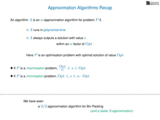
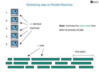
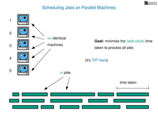
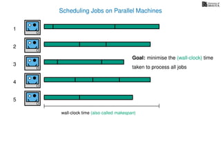
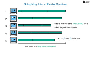
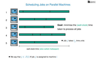
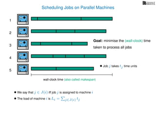
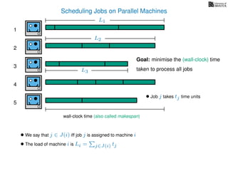
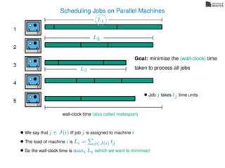
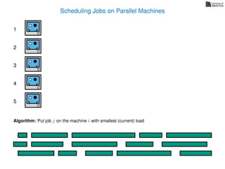
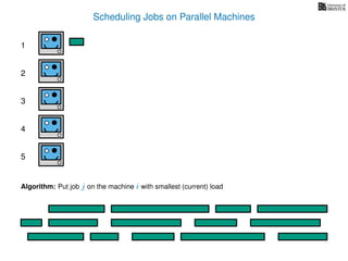
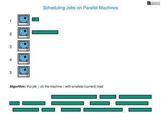
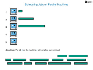
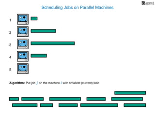
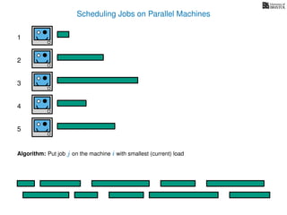
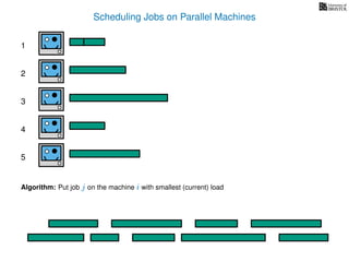
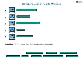
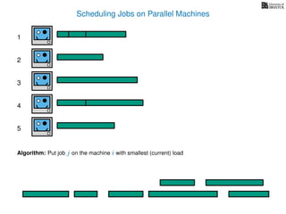
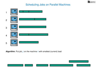
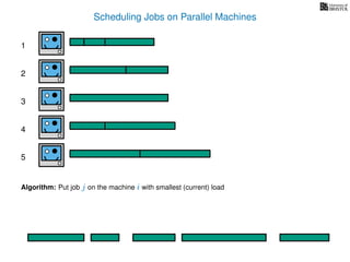
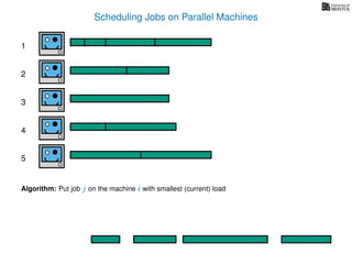
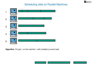
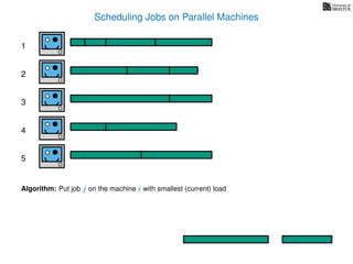
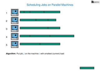
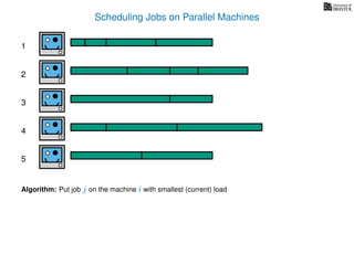
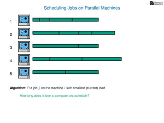
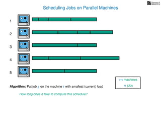
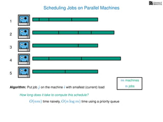
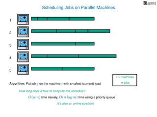
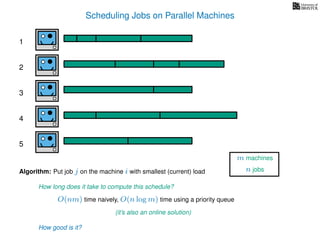
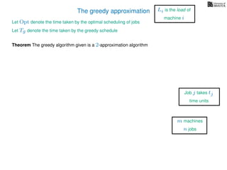
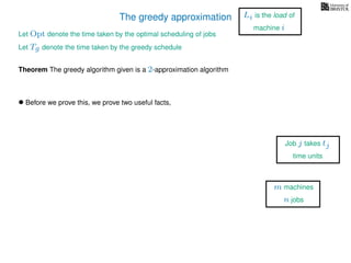
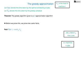
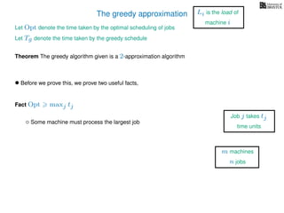
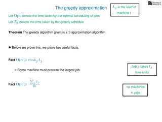
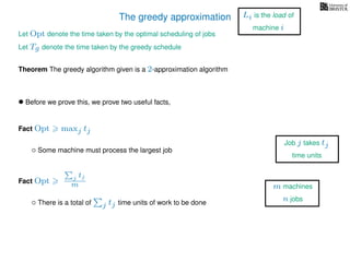
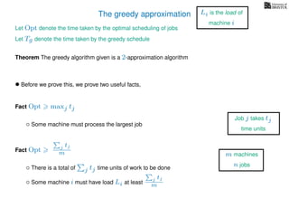
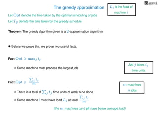
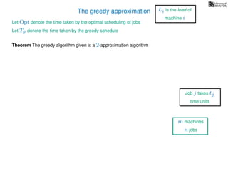
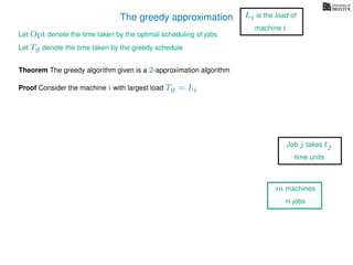
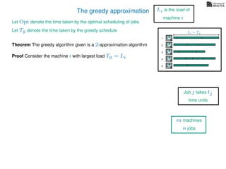
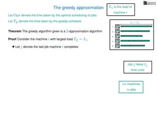
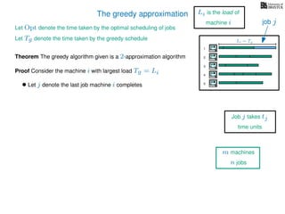
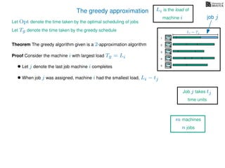
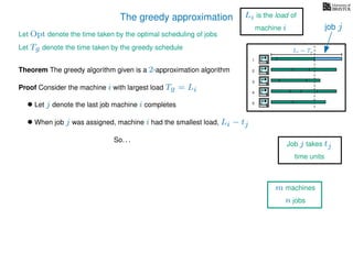
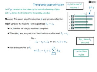
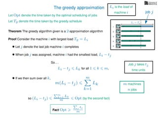
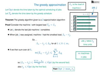
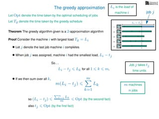
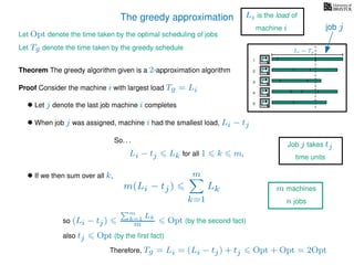
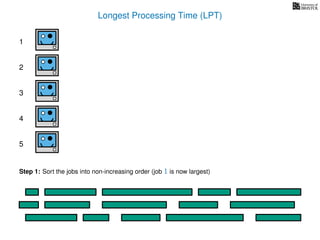
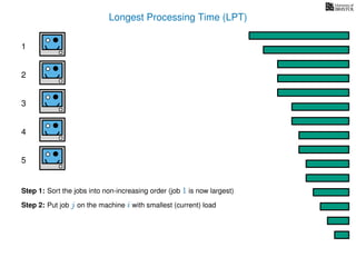
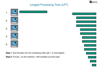
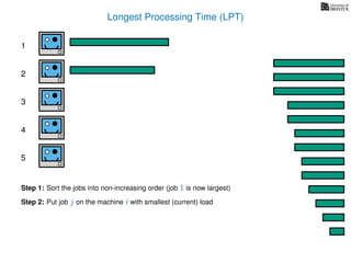
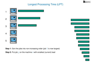
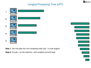
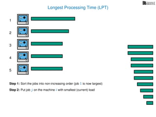
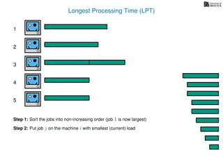
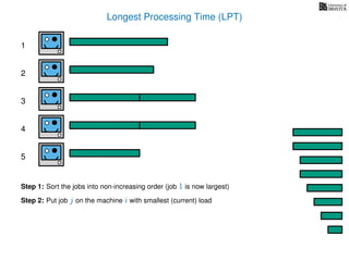
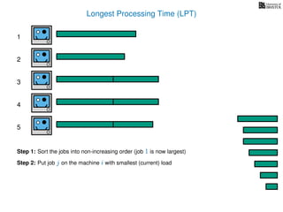
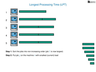
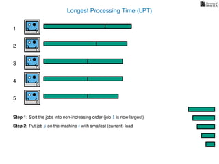
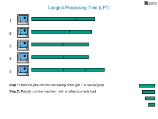
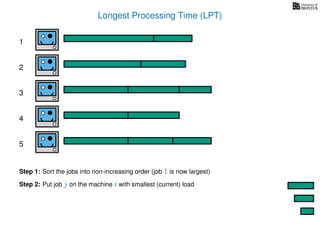
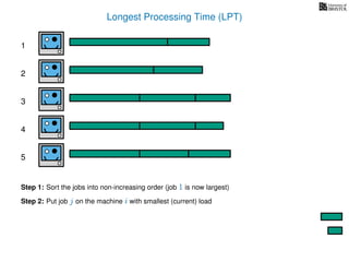
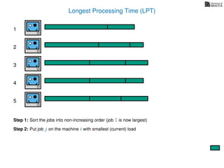
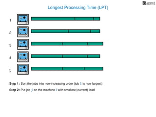
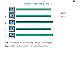
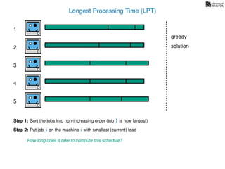
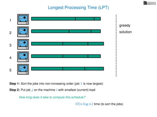
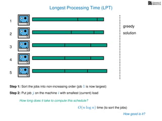
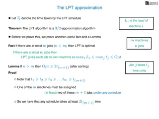
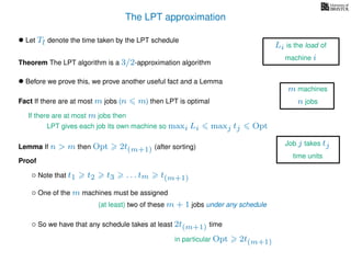
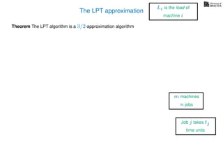
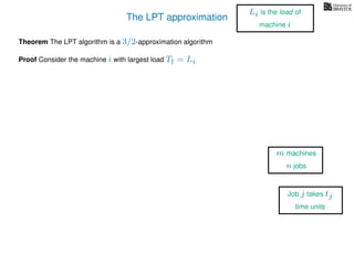
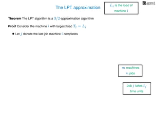
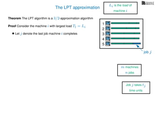
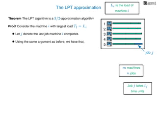
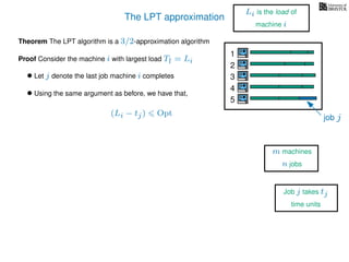
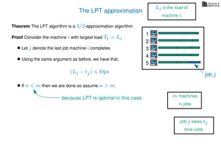
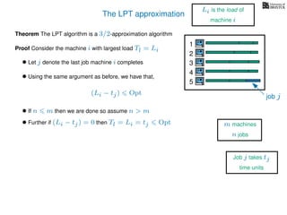
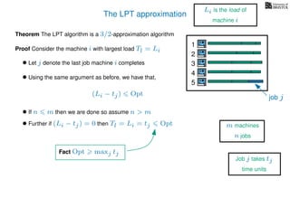
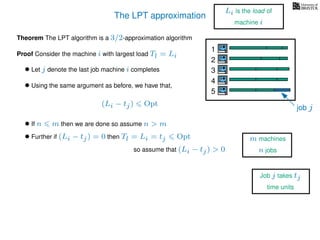
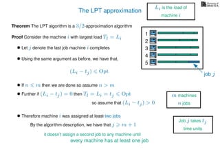
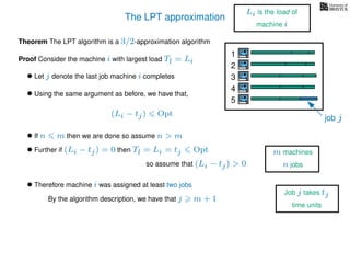
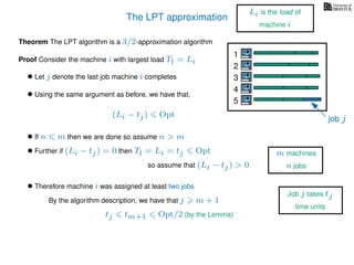
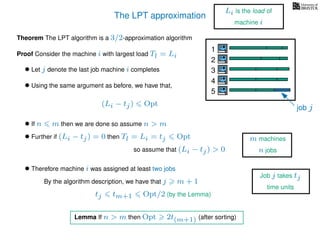
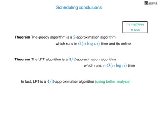
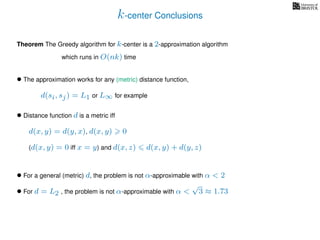
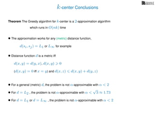
Advanced Algorithms – COMS31900
Approximation algorithms part two
more constant factor approximations
Benjamin Sach
Approximation Algorithms Recap
An algorithm A is an α-approximation algorithm for problem P if,
◦ A runs in polynomial time
◦ A always outputs a solution with value s
Here P is an optimisation problem with optimal solution of value Opt
• If P is a maximisation problem,
Opt
α s Opt
within an α factor of Opt
• If P is a minimisation problem, Opt s α · Opt
We have seen
a 3/2-approximation algorithm for Bin Packing
(and a faster 2-approximation)
Scheduling Jobs on Parallel Machines
1
2
3
4
5
m identical
machines
n jobs
time taken
Goal: minimise the (wall-clock) time
taken to process all jobs
Scheduling Jobs on Parallel Machines
1
2
3
4
5
m identical
machines
n jobs
time taken
Goal: minimise the (wall-clock) time
taken to process all jobs
(it’s NP-hard)
Scheduling Jobs on Parallel Machines
1
2
3
4
5
Goal: minimise the (wall-clock) time
taken to process all jobs
wall-clock time (also called makespan)
Scheduling Jobs on Parallel Machines
1
2
3
4
5
Goal: minimise the (wall-clock) time
taken to process all jobs
wall-clock time (also called makespan)
• Job j takes tj time units
Scheduling Jobs on Parallel Machines
1
2
3
4
5
Goal: minimise the (wall-clock) time
taken to process all jobs
wall-clock time (also called makespan)
• We say that j ∈ J(i) iff job j is assigned to machine i
• Job j takes tj time units
Scheduling Jobs on Parallel Machines
1
2
3
4
5
Goal: minimise the (wall-clock) time
taken to process all jobs
wall-clock time (also called makespan)
• We say that j ∈ J(i) iff job j is assigned to machine i
• The load of machine i is Li = j∈J(i) tj
• Job j takes tj time units
Scheduling Jobs on Parallel Machines
1
2
3
4
5
Goal: minimise the (wall-clock) time
taken to process all jobs
wall-clock time (also called makespan)
• We say that j ∈ J(i) iff job j is assigned to machine i
• The load of machine i is Li = j∈J(i) tj
• Job j takes tj time units
L2
L3
L1
Scheduling Jobs on Parallel Machines
1
2
3
4
5
Goal: minimise the (wall-clock) time
taken to process all jobs
wall-clock time (also called makespan)
• We say that j ∈ J(i) iff job j is assigned to machine i
• The load of machine i is Li = j∈J(i) tj
• Job j takes tj time units
• So the wall-clock time is maxi Li (which we want to minimise)
L2
L3
L1L1
Scheduling Jobs on Parallel Machines
1
2
3
4
5
Scheduling Jobs on Parallel Machines
1
2
3
4
5
Algorithm: Put job j on the machine i with smallest (current) load
Scheduling Jobs on Parallel Machines
1
2
3
4
5
Algorithm: Put job j on the machine i with smallest (current) load
Scheduling Jobs on Parallel Machines
1
2
3
4
5
Algorithm: Put job j on the machine i with smallest (current) load
Scheduling Jobs on Parallel Machines
1
2
3
4
5
Algorithm: Put job j on the machine i with smallest (current) load
Scheduling Jobs on Parallel Machines
1
2
3
4
5
Algorithm: Put job j on the machine i with smallest (current) load
Scheduling Jobs on Parallel Machines
1
2
3
4
5
Algorithm: Put job j on the machine i with smallest (current) load
Scheduling Jobs on Parallel Machines
1
2
3
4
5
Algorithm: Put job j on the machine i with smallest (current) load
Scheduling Jobs on Parallel Machines
1
2
3
4
5
Algorithm: Put job j on the machine i with smallest (current) load
Scheduling Jobs on Parallel Machines
1
2
3
4
5
Algorithm: Put job j on the machine i with smallest (current) load
Scheduling Jobs on Parallel Machines
1
2
3
4
5
Algorithm: Put job j on the machine i with smallest (current) load
Scheduling Jobs on Parallel Machines
1
2
3
4
5
Algorithm: Put job j on the machine i with smallest (current) load
Scheduling Jobs on Parallel Machines
1
2
3
4
5
Algorithm: Put job j on the machine i with smallest (current) load
Scheduling Jobs on Parallel Machines
1
2
3
4
5
Algorithm: Put job j on the machine i with smallest (current) load
Scheduling Jobs on Parallel Machines
1
2
3
4
5
Algorithm: Put job j on the machine i with smallest (current) load
Scheduling Jobs on Parallel Machines
1
2
3
4
5
Algorithm: Put job j on the machine i with smallest (current) load
Scheduling Jobs on Parallel Machines
1
2
3
4
5
Algorithm: Put job j on the machine i with smallest (current) load
Scheduling Jobs on Parallel Machines
1
2
3
4
5
Algorithm: Put job j on the machine i with smallest (current) load
How long does it take to compute this schedule?
Scheduling Jobs on Parallel Machines
1
2
3
4
5
Algorithm: Put job j on the machine i with smallest (current) load
How long does it take to compute this schedule?
m machines
n jobs
Scheduling Jobs on Parallel Machines
1
2
3
4
5
Algorithm: Put job j on the machine i with smallest (current) load
How long does it take to compute this schedule?
O(nm) time naively, O(n log m) time using a priority queue
m machines
n jobs
Scheduling Jobs on Parallel Machines
1
2
3
4
5
Algorithm: Put job j on the machine i with smallest (current) load
How long does it take to compute this schedule?
O(nm) time naively, O(n log m) time using a priority queue
(it’s also an online solution)
m machines
n jobs
Scheduling Jobs on Parallel Machines
1
2
3
4
5
Algorithm: Put job j on the machine i with smallest (current) load
How long does it take to compute this schedule?
O(nm) time naively, O(n log m) time using a priority queue
How good is it?
(it’s also an online solution)
m machines
n jobs
The greedy approximation
Theorem The greedy algorithm given is a 2-approximation algorithm
Let Opt denote the time taken by the optimal scheduling of jobs
Let Tg denote the time taken by the greedy schedule
Job j takes tj
time units
Li is the load of
machine i
m machines
n jobs
The greedy approximation
• Before we prove this, we prove two useful facts,
Fact Opt maxj tj
◦ Some machine must process the largest job
Theorem The greedy algorithm given is a 2-approximation algorithm
Let Opt denote the time taken by the optimal scheduling of jobs
Let Tg denote the time taken by the greedy schedule
Job j takes tj
time units
Li is the load of
machine i
m machines
n jobs
The greedy approximation
• Before we prove this, we prove two useful facts,
Fact Opt maxj tj
Fact Opt j tj
m
◦ Some machine must process the largest job
◦ There is a total of j tj time units of work to be done
◦ Some machine i must have load Li at least
j tj
m
(the m machines can’t all have below average load)
Theorem The greedy algorithm given is a 2-approximation algorithm
Let Opt denote the time taken by the optimal scheduling of jobs
Let Tg denote the time taken by the greedy schedule
Job j takes tj
time units
Li is the load of
machine i
m machines
n jobs
The greedy approximation
Theorem The greedy algorithm given is a 2-approximation algorithm
Let Opt denote the time taken by the optimal scheduling of jobs
Let Tg denote the time taken by the greedy schedule
Li is the load of
machine i
Job j takes tj
time units
m machines
n jobs
The greedy approximation
Theorem The greedy algorithm given is a 2-approximation algorithm
Proof Consider the machine i with largest load Tg = Li
Let Opt denote the time taken by the optimal scheduling of jobs
Let Tg denote the time taken by the greedy schedule
Li is the load of
machine i
Job j takes tj
time units
1
2
3
4
5
Li = Tg
m machines
n jobs
The greedy approximation
Theorem The greedy algorithm given is a 2-approximation algorithm
• Let j denote the last job machine i completes
Proof Consider the machine i with largest load Tg = Li
Let Opt denote the time taken by the optimal scheduling of jobs
Let Tg denote the time taken by the greedy schedule
Li is the load of
machine i
Job j takes tj
time units
1
2
3
4
5
Li = Tg
m machines
n jobs
job j
The greedy approximation
Theorem The greedy algorithm given is a 2-approximation algorithm
• Let j denote the last job machine i completes
Proof Consider the machine i with largest load Tg = Li
• When job j was assigned, machine i had the smallest load, Li − tj
Let Opt denote the time taken by the optimal scheduling of jobs
Let Tg denote the time taken by the greedy schedule
Li is the load of
machine i
Job j takes tj
time units
1
2
3
4
5
Li = Tg
m machines
n jobs
job j
The greedy approximation
Theorem The greedy algorithm given is a 2-approximation algorithm
• Let j denote the last job machine i completes
Proof Consider the machine i with largest load Tg = Li
• When job j was assigned, machine i had the smallest load, Li − tj
So. . .
Let Opt denote the time taken by the optimal scheduling of jobs
Let Tg denote the time taken by the greedy schedule
Li is the load of
machine i
Job j takes tj
time units
1
2
3
4
5
Li = Tg
m machines
n jobs
job j
The greedy approximation
Theorem The greedy algorithm given is a 2-approximation algorithm
• Let j denote the last job machine i completes
Proof Consider the machine i with largest load Tg = Li
• When job j was assigned, machine i had the smallest load, Li − tj
Li − tj Lk for all 1 k m,
So. . .
• If we then sum over all k,
m(Li − tj)
m
k=1
Lk
so (Li − tj)
m
k=1 Lk
m Opt (by the second fact)
Let Opt denote the time taken by the optimal scheduling of jobs
Let Tg denote the time taken by the greedy schedule
Li is the load of
machine i
Job j takes tj
time units
1
2
3
4
5
Li = Tg
m machines
n jobs
job j
Fact Opt j tj
m
The greedy approximation
Theorem The greedy algorithm given is a 2-approximation algorithm
• Let j denote the last job machine i completes
Proof Consider the machine i with largest load Tg = Li
• When job j was assigned, machine i had the smallest load, Li − tj
Li − tj Lk for all 1 k m,
So. . .
• If we then sum over all k,
m(Li − tj)
m
k=1
Lk
so (Li − tj)
m
k=1 Lk
m Opt (by the second fact)
Let Opt denote the time taken by the optimal scheduling of jobs
Let Tg denote the time taken by the greedy schedule
Li is the load of
machine i
Job j takes tj
time units
1
2
3
4
5
Li = Tg
m machines
n jobs
job j
The greedy approximation
Theorem The greedy algorithm given is a 2-approximation algorithm
• Let j denote the last job machine i completes
Proof Consider the machine i with largest load Tg = Li
• When job j was assigned, machine i had the smallest load, Li − tj
Li − tj Lk for all 1 k m,
So. . .
• If we then sum over all k,
m(Li − tj)
m
k=1
Lk
so (Li − tj)
m
k=1 Lk
m Opt (by the second fact)
also tj Opt (by the first fact)
Let Opt denote the time taken by the optimal scheduling of jobs
Let Tg denote the time taken by the greedy schedule
Li is the load of
machine i
Job j takes tj
time units
1
2
3
4
5
Li = Tg
m machines
n jobs
job j
Fact Opt maxj tj
The greedy approximation
Theorem The greedy algorithm given is a 2-approximation algorithm
• Let j denote the last job machine i completes
Proof Consider the machine i with largest load Tg = Li
• When job j was assigned, machine i had the smallest load, Li − tj
Li − tj Lk for all 1 k m,
So. . .
• If we then sum over all k,
m(Li − tj)
m
k=1
Lk
so (Li − tj)
m
k=1 Lk
m Opt (by the second fact)
also tj Opt (by the first fact)
Let Opt denote the time taken by the optimal scheduling of jobs
Let Tg denote the time taken by the greedy schedule
Li is the load of
machine i
Job j takes tj
time units
1
2
3
4
5
Li = Tg
m machines
n jobs
job j
The greedy approximation
Theorem The greedy algorithm given is a 2-approximation algorithm
• Let j denote the last job machine i completes
Proof Consider the machine i with largest load Tg = Li
• When job j was assigned, machine i had the smallest load, Li − tj
Li − tj Lk for all 1 k m,
So. . .
• If we then sum over all k,
m(Li − tj)
m
k=1
Lk
so (Li − tj)
m
k=1 Lk
m Opt (by the second fact)
also tj Opt (by the first fact)
Therefore, Tg = Li = (Li − tj) + tj Opt + Opt = 2Opt
Let Opt denote the time taken by the optimal scheduling of jobs
Let Tg denote the time taken by the greedy schedule
Li is the load of
machine i
Job j takes tj
time units
1
2
3
4
5
Li = Tg
m machines
n jobs
job j
Longest Processing Time (LPT)
1
2
3
4
5
Step 1: Sort the jobs into non-increasing order (job 1 is now largest)
Longest Processing Time (LPT)
1
2
3
4
5
Step 1: Sort the jobs into non-increasing order (job 1 is now largest)
Longest Processing Time (LPT)
1
2
3
4
5
Step 1: Sort the jobs into non-increasing order (job 1 is now largest)
Step 2: Put job j on the machine i with smallest (current) load
Longest Processing Time (LPT)
1
2
3
4
5
Step 1: Sort the jobs into non-increasing order (job 1 is now largest)
Step 2: Put job j on the machine i with smallest (current) load
Longest Processing Time (LPT)
1
2
3
4
5
Step 1: Sort the jobs into non-increasing order (job 1 is now largest)
Step 2: Put job j on the machine i with smallest (current) load
Longest Processing Time (LPT)
1
2
3
4
5
Step 1: Sort the jobs into non-increasing order (job 1 is now largest)
Step 2: Put job j on the machine i with smallest (current) load
Longest Processing Time (LPT)
1
2
3
4
5
Step 1: Sort the jobs into non-increasing order (job 1 is now largest)
Step 2: Put job j on the machine i with smallest (current) load
Longest Processing Time (LPT)
1
2
3
4
5
Step 1: Sort the jobs into non-increasing order (job 1 is now largest)
Step 2: Put job j on the machine i with smallest (current) load
Longest Processing Time (LPT)
1
2
3
4
5
Step 1: Sort the jobs into non-increasing order (job 1 is now largest)
Step 2: Put job j on the machine i with smallest (current) load
Longest Processing Time (LPT)
1
2
3
4
5
Step 1: Sort the jobs into non-increasing order (job 1 is now largest)
Step 2: Put job j on the machine i with smallest (current) load
Longest Processing Time (LPT)
1
2
3
4
5
Step 1: Sort the jobs into non-increasing order (job 1 is now largest)
Step 2: Put job j on the machine i with smallest (current) load
Longest Processing Time (LPT)
1
2
3
4
5
Step 1: Sort the jobs into non-increasing order (job 1 is now largest)
Step 2: Put job j on the machine i with smallest (current) load
Longest Processing Time (LPT)
1
2
3
4
5
Step 1: Sort the jobs into non-increasing order (job 1 is now largest)
Step 2: Put job j on the machine i with smallest (current) load
Longest Processing Time (LPT)
1
2
3
4
5
Step 1: Sort the jobs into non-increasing order (job 1 is now largest)
Step 2: Put job j on the machine i with smallest (current) load
Longest Processing Time (LPT)
1
2
3
4
5
Step 1: Sort the jobs into non-increasing order (job 1 is now largest)
Step 2: Put job j on the machine i with smallest (current) load
Longest Processing Time (LPT)
1
2
3
4
5
Step 1: Sort the jobs into non-increasing order (job 1 is now largest)
Step 2: Put job j on the machine i with smallest (current) load
Longest Processing Time (LPT)
1
2
3
4
5
Step 1: Sort the jobs into non-increasing order (job 1 is now largest)
Step 2: Put job j on the machine i with smallest (current) load
Longest Processing Time (LPT)
1
2
3
4
5
Step 1: Sort the jobs into non-increasing order (job 1 is now largest)
Step 2: Put job j on the machine i with smallest (current) load
Longest Processing Time (LPT)
1
2
3
4
5
Step 1: Sort the jobs into non-increasing order (job 1 is now largest)
Step 2: Put job j on the machine i with smallest (current) load
greedy
solution
Longest Processing Time (LPT)
1
2
3
4
5
Step 1: Sort the jobs into non-increasing order (job 1 is now largest)
Step 2: Put job j on the machine i with smallest (current) load
greedy
solution
How long does it take to compute this schedule?
Longest Processing Time (LPT)
1
2
3
4
5
Step 1: Sort the jobs into non-increasing order (job 1 is now largest)
Step 2: Put job j on the machine i with smallest (current) load
greedy
solution
How long does it take to compute this schedule?
O(n log n) time (to sort the jobs)
Longest Processing Time (LPT)
1
2
3
4
5
Step 1: Sort the jobs into non-increasing order (job 1 is now largest)
Step 2: Put job j on the machine i with smallest (current) load
greedy
solution
How long does it take to compute this schedule?
O(n log n) time (to sort the jobs)
How good is it?
The LPT approximation
Theorem The LPT algorithm is a 3/2-approximation algorithm
• Let Tl denote the time taken by the LPT schedule
Li is the load of
machine i
m machines
n jobs
Job j takes tj
time units
The LPT approximation
Theorem The LPT algorithm is a 3/2-approximation algorithm
• Before we prove this, we prove another useful fact and a Lemma
• Let Tl denote the time taken by the LPT schedule
Li is the load of
machine i
m machines
n jobs
Job j takes tj
time units
The LPT approximation
Theorem The LPT algorithm is a 3/2-approximation algorithm
• Before we prove this, we prove another useful fact and a Lemma
Fact If there are at most m jobs (n m) then LPT is optimal
LPT gives each job its own machine so maxi Li maxj tj Opt
• Let Tl denote the time taken by the LPT schedule
Li is the load of
machine i
m machines
n jobs
Job j takes tj
time units
If there are at most m jobs then
The LPT approximation
Theorem The LPT algorithm is a 3/2-approximation algorithm
• Before we prove this, we prove another useful fact and a Lemma
Fact If there are at most m jobs (n m) then LPT is optimal
Lemma If n > m then Opt 2t(m+1) (after sorting)
LPT gives each job its own machine so maxi Li maxj tj Opt
• Let Tl denote the time taken by the LPT schedule
Proof
Li is the load of
machine i
m machines
n jobs
Job j takes tj
time units
If there are at most m jobs then
The LPT approximation
Theorem The LPT algorithm is a 3/2-approximation algorithm
• Before we prove this, we prove another useful fact and a Lemma
Fact If there are at most m jobs (n m) then LPT is optimal
Lemma If n > m then Opt 2t(m+1) (after sorting)
LPT gives each job its own machine so maxi Li maxj tj Opt
◦ Note that t1 t2 t3 . . . tm t(m+1)
◦ One of the m machines must be assigned
• Let Tl denote the time taken by the LPT schedule
Proof
(at least) two of these m + 1 jobs under any schedule
◦ So we have that any schedule takes at least 2t(m+1) time
Li is the load of
machine i
m machines
n jobs
in particular Opt 2t(m+1)
Job j takes tj
time units
If there are at most m jobs then
The LPT approximation
Theorem The LPT algorithm is a 3/2-approximation algorithm
Li is the load of
machine i
m machines
n jobs
Job j takes tj
time units
The LPT approximation
Theorem The LPT algorithm is a 3/2-approximation algorithm
Proof Consider the machine i with largest load Tl = Li
Li is the load of
machine i
m machines
n jobs
Job j takes tj
time units
The LPT approximation
Theorem The LPT algorithm is a 3/2-approximation algorithm
• Let j denote the last job machine i completes
Proof Consider the machine i with largest load Tl = Li
Li is the load of
machine i
m machines
n jobs
Job j takes tj
time units
The LPT approximation
Theorem The LPT algorithm is a 3/2-approximation algorithm
• Let j denote the last job machine i completes
Proof Consider the machine i with largest load Tl = Li
Li is the load of
machine i
m machines
n jobs
Job j takes tj
time units
job j
1
2
3
4
5
The LPT approximation
Theorem The LPT algorithm is a 3/2-approximation algorithm
• Let j denote the last job machine i completes
Proof Consider the machine i with largest load Tl = Li
• Using the same argument as before, we have that,
(Li − tj) Opt
• If n m then we are done so assume n > m
Li is the load of
machine i
m machines
n jobs
Job j takes tj
time units
job j
1
2
3
4
5
because LPT is optimal in this case
The LPT approximation
Theorem The LPT algorithm is a 3/2-approximation algorithm
• Let j denote the last job machine i completes
Proof Consider the machine i with largest load Tl = Li
• Using the same argument as before, we have that,
(Li − tj) Opt
• If n m then we are done so assume n > m
Li is the load of
machine i
m machines
n jobs
Job j takes tj
time units
job j
1
2
3
4
5
The LPT approximation
Theorem The LPT algorithm is a 3/2-approximation algorithm
• Let j denote the last job machine i completes
Proof Consider the machine i with largest load Tl = Li
• Using the same argument as before, we have that,
(Li − tj) Opt
• If n m then we are done so assume n > m
• Further if (Li − tj) = 0 then Tl = Li = tj Opt
Li is the load of
machine i
m machines
n jobs
Job j takes tj
time units
job j
1
2
3
4
5
Fact Opt maxj tj
The LPT approximation
Theorem The LPT algorithm is a 3/2-approximation algorithm
• Let j denote the last job machine i completes
Proof Consider the machine i with largest load Tl = Li
• Using the same argument as before, we have that,
(Li − tj) Opt
• If n m then we are done so assume n > m
• Further if (Li − tj) = 0 then Tl = Li = tj Opt
Li is the load of
machine i
m machines
n jobs
Job j takes tj
time units
job j
1
2
3
4
5
The LPT approximation
Theorem The LPT algorithm is a 3/2-approximation algorithm
• Let j denote the last job machine i completes
Proof Consider the machine i with largest load Tl = Li
• Using the same argument as before, we have that,
(Li − tj) Opt
• If n m then we are done so assume n > m
• Further if (Li − tj) = 0 then Tl = Li = tj Opt
so assume that (Li − tj) > 0
• Therefore machine i was assigned at least two jobs
By the algorithm description, we have that j m + 1
Li is the load of
machine i
m machines
n jobs
Job j takes tj
time units
job j
1
2
3
4
5
it doesn’t assign a second job to any machine until
every machine has at least one job
The LPT approximation
Theorem The LPT algorithm is a 3/2-approximation algorithm
• Let j denote the last job machine i completes
Proof Consider the machine i with largest load Tl = Li
• Using the same argument as before, we have that,
(Li − tj) Opt
• If n m then we are done so assume n > m
• Further if (Li − tj) = 0 then Tl = Li = tj Opt
so assume that (Li − tj) > 0
• Therefore machine i was assigned at least two jobs
By the algorithm description, we have that j m + 1
Li is the load of
machine i
m machines
n jobs
Job j takes tj
time units
job j
1
2
3
4
5
The LPT approximation
Theorem The LPT algorithm is a 3/2-approximation algorithm
• Let j denote the last job machine i completes
Proof Consider the machine i with largest load Tl = Li
• Using the same argument as before, we have that,
(Li − tj) Opt
• If n m then we are done so assume n > m
• Further if (Li − tj) = 0 then Tl = Li = tj Opt
so assume that (Li − tj) > 0
• Therefore machine i was assigned at least two jobs
By the algorithm description, we have that j m + 1
tj tm+1 Opt/2 (by the Lemma)
Li is the load of
machine i
m machines
n jobs
Job j takes tj
time units
job j
1
2
3
4
5
Lemma If n > m then Opt 2t(m+1) (after sorting)
The LPT approximation
Theorem The LPT algorithm is a 3/2-approximation algorithm
• Let j denote the last job machine i completes
Proof Consider the machine i with largest load Tl = Li
• Using the same argument as before, we have that,
(Li − tj) Opt
• If n m then we are done so assume n > m
• Further if (Li − tj) = 0 then Tl = Li = tj Opt
so assume that (Li − tj) > 0
• Therefore machine i was assigned at least two jobs
By the algorithm description, we have that j m + 1
tj tm+1 Opt/2 (by the Lemma)
Li is the load of
machine i
m machines
n jobs
Job j takes tj
time units
job j
1
2
3
4
5
The LPT approximation
Theorem The LPT algorithm is a 3/2-approximation algorithm
• Let j denote the last job machine i completes
Proof Consider the machine i with largest load Tl = Li
• Using the same argument as before, we have that,
(Li − tj) Opt
Therefore, Tl = Li = (Li − tj) + tj Opt + Opt/2 = (3/2) · Opt
• If n m then we are done so assume n > m
• Further if (Li − tj) = 0 then Tl = Li = tj Opt
so assume that (Li − tj) > 0
• Therefore machine i was assigned at least two jobs
By the algorithm description, we have that j m + 1
tj tm+1 Opt/2 (by the Lemma)
Li is the load of
machine i
m machines
n jobs
Job j takes tj
time units
job j
1
2
3
4
5
Scheduling conclusions
Theorem The LPT algorithm is a 3/2-approximation algorithm
which runs in O(n log n) time
Theorem The greedy algorithm is a 2-approximation algorithm
which runs in O(n log m) time and it’s online
In fact, LPT is a 4/3-approximation algorithm (using better analysis)
m machines
n jobs
k-centers
k-centers
k-centers
n points (sites) in 2D space
k-centers
n points (sites) in 2D space
The distance between points si, sj is (xi − xj)2 + (yi − yj)2
k-centers
n points (sites) in 2D space
The distance between points si, sj is (xi − xj)2 + (yi − yj)2
(i.e. ‘normal’ euclidean distance)
k-centers
n points (sites) in 2D space
The distance between points si, sj is (xi − xj)2 + (yi − yj)2
Select k sites to be
centers
(i.e. ‘normal’ euclidean distance)
k-centers
n points (sites) in 2D space
The distance between points si, sj is (xi − xj)2 + (yi − yj)2
Select k sites to be
centers
(i.e. ‘normal’ euclidean distance)
k-centers
n points (sites) in 2D space
The distance between points si, sj is (xi − xj)2 + (yi − yj)2
Select k sites to be
centers
k-centers
n points (sites) in 2D space
The distance between points si, sj is (xi − xj)2 + (yi − yj)2
Goal Minimise the largest distance from any site to the closest center
Select k sites to be
centers
k-centers
n points (sites) in 2D space
The distance between points si, sj is (xi − xj)2 + (yi − yj)2
Goal Minimise the largest distance from any site to the closest center
Select k sites to be
centers
k-centers
n points (sites) in 2D space
The distance between points si, sj is (xi − xj)2 + (yi − yj)2
Goal Minimise the largest distance from any site to the closest center
Select k sites to be
centers
r
r
k-centers
n points (sites) in 2D space
The distance between points si, sj is (xi − xj)2 + (yi − yj)2
Goal Minimise the largest distance from any site to the closest center
Select k sites to be
centers
k-centers
n points (sites) in 2D space
The distance between points si, sj is (xi − xj)2 + (yi − yj)2
Goal Minimise the largest distance from any site to the closest center
Select k sites to be
centers
k-centers
n points (sites) in 2D space
The distance between points si, sj is (xi − xj)2 + (yi − yj)2
Goal Minimise the largest distance from any site to the closest center
Select k sites to be
centers
r
k-centers
n points (sites) in 2D space
The distance between points si, sj is (xi − xj)2 + (yi − yj)2
Goal Minimise the largest distance from any site to the closest center
(in general it’s NP-hard)
Select k sites to be
centers
r
A Greedy approximation
Start by picking any point to be a center
A Greedy approximation
Start by picking any point to be a center
A Greedy approximation
Start by picking any point to be a center
Repeatedly pick the site which is furthest from any existing center
A Greedy approximation
Start by picking any point to be a center
Repeatedly pick the site which is furthest from any existing center
A Greedy approximation
Start by picking any point to be a center
Repeatedly pick the site which is furthest from any existing center
A Greedy approximation
Start by picking any point to be a center
Repeatedly pick the site which is furthest from any existing center
A Greedy approximation
Start by picking any point to be a center
Repeatedly pick the site which is furthest from any existing center
A Greedy approximation
Start by picking any point to be a center
Repeatedly pick the site which is furthest from any existing center
A Greedy approximation
Start by picking any point to be a center
Repeatedly pick the site which is furthest from any existing center
A Greedy approximation
Start by picking any point to be a center
Repeatedly pick the site which is furthest from any existing center
A Greedy approximation
Start by picking any point to be a center
Repeatedly pick the site which is furthest from any existing center
A Greedy approximation
Start by picking any point to be a center
Repeatedly pick the site which is furthest from any existing center
A Greedy approximation
Start by picking any point to be a center
Repeatedly pick the site which is furthest from any existing center
A Greedy approximation
Start by picking any point to be a center
Repeatedly pick the site which is furthest from any existing center
A Greedy approximation
Start by picking any point to be a center
Repeatedly pick the site which is furthest from any existing center
A Greedy approximation
Start by picking any point to be a center
Repeatedly pick the site which is furthest from any existing center
A Greedy approximation
Start by picking any point to be a center
Repeatedly pick the site which is furthest from any existing center
A Greedy approximation
r
Start by picking any point to be a center
Repeatedly pick the site which is furthest from any existing center
This takes O(nk) time
A Greedy approximation
Start by picking any point to be a center
Repeatedly pick the site which is furthest from any existing center
This takes O(nk) time
A Greedy approximation
but is it any good?
The Greedy approximation
Theorem The Greedy algorithm for k-center is a 2-approximation algorithm
Let Cg (resp. COpt) denote the set of centers selected by Greedy (resp. Optimal)
Proof
Let rg (resp. Opt) denote largest site-center distance using Greedy (resp. Optimal)
The Greedy approximation
Theorem The Greedy algorithm for k-center is a 2-approximation algorithm
Let Cg (resp. COpt) denote the set of centers selected by Greedy (resp. Optimal)
Proof
Let rg (resp. Opt) denote largest site-center distance using Greedy (resp. Optimal)
Case 1: No si, si ∈ Cg are closest to the same sj ∈ COpt
Optimal centers
Opt
Sites
purposes only
Disclaimer: for illustrative
Greedy centers
Distance at most 2Opt
so rg 2Opt
The Greedy approximation
Theorem The Greedy algorithm for k-center is a 2-approximation algorithm
Let Cg (resp. COpt) denote the set of centers selected by Greedy (resp. Optimal)
Proof
Let rg (resp. Opt) denote largest site-center distance using Greedy (resp. Optimal)
Case 2: Some si, si ∈ Cg are closest to the same sj ∈ COpt
si
si
The Greedy approximation
Theorem The Greedy algorithm for k-center is a 2-approximation algorithm
Let Cg (resp. COpt) denote the set of centers selected by Greedy (resp. Optimal)
Proof
Let rg (resp. Opt) denote largest site-center distance using Greedy (resp. Optimal)
Case 2: Some si, si ∈ Cg are closest to the same sj ∈ COpt
Assume wlog. that Greedy made si a center after si
si
si
si was added as a center because it was
the furthest from any existing Greedy center
However, si is at most 2Opt away from si
So even before adding si as a center, all sites
were 2Opt away from a Greedy center
Therefore, rg 2Opt
k-center Conclusions
Theorem The Greedy algorithm for k-center is a 2-approximation algorithm
which runs in O(nk) time
k-center Conclusions
Theorem The Greedy algorithm for k-center is a 2-approximation algorithm
which runs in O(nk) time
• The approximation works for any (metric) distance function,
k-center Conclusions
Theorem The Greedy algorithm for k-center is a 2-approximation algorithm
which runs in O(nk) time
• The approximation works for any (metric) distance function,
d(si, sj) = L1 or L∞ for example
k-center Conclusions
Theorem The Greedy algorithm for k-center is a 2-approximation algorithm
which runs in O(nk) time
• The approximation works for any (metric) distance function,
d(si, sj) = L1 or L∞ for example
d(x, y) = d(y, x), d(x, y) 0
• Distance function d is a metric iff
(d(x, y) = 0 iff x = y) and d(x, z) d(x, y) + d(y, z)
k-center Conclusions
Theorem The Greedy algorithm for k-center is a 2-approximation algorithm
which runs in O(nk) time
• The approximation works for any (metric) distance function,
d(si, sj) = L1 or L∞ for example
• For a general (metric) d, the problem is not α-approximable with α < 2
d(x, y) = d(y, x), d(x, y) 0
• For d = L2 , the problem is not α-approximable with α <
√
3 ≈ 1.73
• For d = L1 or d = L∞ , the problem is not α-approximable with α < 2
• Distance function d is a metric iff
(d(x, y) = 0 iff x = y) and d(x, z) d(x, y) + d(y, z)

Approximation Algorithms Part Two: More Constant factor approximations

  • 1.
    Advanced Algorithms –COMS31900 Approximation algorithms part two more constant factor approximations Benjamin Sach
  • 2.
    Approximation Algorithms Recap Analgorithm A is an α-approximation algorithm for problem P if, ◦ A runs in polynomial time ◦ A always outputs a solution with value s Here P is an optimisation problem with optimal solution of value Opt • If P is a maximisation problem, Opt α s Opt within an α factor of Opt • If P is a minimisation problem, Opt s α · Opt We have seen a 3/2-approximation algorithm for Bin Packing (and a faster 2-approximation)
  • 3.
    Scheduling Jobs onParallel Machines 1 2 3 4 5 m identical machines n jobs time taken Goal: minimise the (wall-clock) time taken to process all jobs
  • 4.
    Scheduling Jobs onParallel Machines 1 2 3 4 5 m identical machines n jobs time taken Goal: minimise the (wall-clock) time taken to process all jobs (it’s NP-hard)
  • 5.
    Scheduling Jobs onParallel Machines 1 2 3 4 5 Goal: minimise the (wall-clock) time taken to process all jobs wall-clock time (also called makespan)
  • 6.
    Scheduling Jobs onParallel Machines 1 2 3 4 5 Goal: minimise the (wall-clock) time taken to process all jobs wall-clock time (also called makespan) • Job j takes tj time units
  • 7.
    Scheduling Jobs onParallel Machines 1 2 3 4 5 Goal: minimise the (wall-clock) time taken to process all jobs wall-clock time (also called makespan) • We say that j ∈ J(i) iff job j is assigned to machine i • Job j takes tj time units
  • 8.
    Scheduling Jobs onParallel Machines 1 2 3 4 5 Goal: minimise the (wall-clock) time taken to process all jobs wall-clock time (also called makespan) • We say that j ∈ J(i) iff job j is assigned to machine i • The load of machine i is Li = j∈J(i) tj • Job j takes tj time units
  • 9.
    Scheduling Jobs onParallel Machines 1 2 3 4 5 Goal: minimise the (wall-clock) time taken to process all jobs wall-clock time (also called makespan) • We say that j ∈ J(i) iff job j is assigned to machine i • The load of machine i is Li = j∈J(i) tj • Job j takes tj time units L2 L3 L1
  • 10.
    Scheduling Jobs onParallel Machines 1 2 3 4 5 Goal: minimise the (wall-clock) time taken to process all jobs wall-clock time (also called makespan) • We say that j ∈ J(i) iff job j is assigned to machine i • The load of machine i is Li = j∈J(i) tj • Job j takes tj time units • So the wall-clock time is maxi Li (which we want to minimise) L2 L3 L1
  • 11.
    Scheduling Jobs onParallel Machines 1 2 3 4 5 Goal: minimise the (wall-clock) time taken to process all jobs wall-clock time (also called makespan) • We say that j ∈ J(i) iff job j is assigned to machine i • The load of machine i is Li = j∈J(i) tj • Job j takes tj time units • So the wall-clock time is maxi Li (which we want to minimise) L2 L3 L1L1
  • 12.
    Scheduling Jobs onParallel Machines 1 2 3 4 5
  • 13.
    Scheduling Jobs onParallel Machines 1 2 3 4 5 Algorithm: Put job j on the machine i with smallest (current) load
  • 14.
    Scheduling Jobs onParallel Machines 1 2 3 4 5 Algorithm: Put job j on the machine i with smallest (current) load
  • 15.
    Scheduling Jobs onParallel Machines 1 2 3 4 5 Algorithm: Put job j on the machine i with smallest (current) load
  • 16.
    Scheduling Jobs onParallel Machines 1 2 3 4 5 Algorithm: Put job j on the machine i with smallest (current) load
  • 17.
    Scheduling Jobs onParallel Machines 1 2 3 4 5 Algorithm: Put job j on the machine i with smallest (current) load
  • 18.
    Scheduling Jobs onParallel Machines 1 2 3 4 5 Algorithm: Put job j on the machine i with smallest (current) load
  • 19.
    Scheduling Jobs onParallel Machines 1 2 3 4 5 Algorithm: Put job j on the machine i with smallest (current) load
  • 20.
    Scheduling Jobs onParallel Machines 1 2 3 4 5 Algorithm: Put job j on the machine i with smallest (current) load
  • 21.
    Scheduling Jobs onParallel Machines 1 2 3 4 5 Algorithm: Put job j on the machine i with smallest (current) load
  • 22.
    Scheduling Jobs onParallel Machines 1 2 3 4 5 Algorithm: Put job j on the machine i with smallest (current) load
  • 23.
    Scheduling Jobs onParallel Machines 1 2 3 4 5 Algorithm: Put job j on the machine i with smallest (current) load
  • 24.
    Scheduling Jobs onParallel Machines 1 2 3 4 5 Algorithm: Put job j on the machine i with smallest (current) load
  • 25.
    Scheduling Jobs onParallel Machines 1 2 3 4 5 Algorithm: Put job j on the machine i with smallest (current) load
  • 26.
    Scheduling Jobs onParallel Machines 1 2 3 4 5 Algorithm: Put job j on the machine i with smallest (current) load
  • 27.
    Scheduling Jobs onParallel Machines 1 2 3 4 5 Algorithm: Put job j on the machine i with smallest (current) load
  • 28.
    Scheduling Jobs onParallel Machines 1 2 3 4 5 Algorithm: Put job j on the machine i with smallest (current) load
  • 29.
    Scheduling Jobs onParallel Machines 1 2 3 4 5 Algorithm: Put job j on the machine i with smallest (current) load How long does it take to compute this schedule?
  • 30.
    Scheduling Jobs onParallel Machines 1 2 3 4 5 Algorithm: Put job j on the machine i with smallest (current) load How long does it take to compute this schedule? m machines n jobs
  • 31.
    Scheduling Jobs onParallel Machines 1 2 3 4 5 Algorithm: Put job j on the machine i with smallest (current) load How long does it take to compute this schedule? O(nm) time naively, O(n log m) time using a priority queue m machines n jobs
  • 32.
    Scheduling Jobs onParallel Machines 1 2 3 4 5 Algorithm: Put job j on the machine i with smallest (current) load How long does it take to compute this schedule? O(nm) time naively, O(n log m) time using a priority queue (it’s also an online solution) m machines n jobs
  • 33.
    Scheduling Jobs onParallel Machines 1 2 3 4 5 Algorithm: Put job j on the machine i with smallest (current) load How long does it take to compute this schedule? O(nm) time naively, O(n log m) time using a priority queue How good is it? (it’s also an online solution) m machines n jobs
  • 34.
    The greedy approximation TheoremThe greedy algorithm given is a 2-approximation algorithm Let Opt denote the time taken by the optimal scheduling of jobs Let Tg denote the time taken by the greedy schedule Job j takes tj time units Li is the load of machine i m machines n jobs
  • 35.
    The greedy approximation •Before we prove this, we prove two useful facts, Theorem The greedy algorithm given is a 2-approximation algorithm Let Opt denote the time taken by the optimal scheduling of jobs Let Tg denote the time taken by the greedy schedule Job j takes tj time units Li is the load of machine i m machines n jobs
  • 36.
    The greedy approximation •Before we prove this, we prove two useful facts, Fact Opt maxj tj Theorem The greedy algorithm given is a 2-approximation algorithm Let Opt denote the time taken by the optimal scheduling of jobs Let Tg denote the time taken by the greedy schedule Job j takes tj time units Li is the load of machine i m machines n jobs
  • 37.
    The greedy approximation •Before we prove this, we prove two useful facts, Fact Opt maxj tj ◦ Some machine must process the largest job Theorem The greedy algorithm given is a 2-approximation algorithm Let Opt denote the time taken by the optimal scheduling of jobs Let Tg denote the time taken by the greedy schedule Job j takes tj time units Li is the load of machine i m machines n jobs
  • 38.
    The greedy approximation •Before we prove this, we prove two useful facts, Fact Opt maxj tj Fact Opt j tj m ◦ Some machine must process the largest job Theorem The greedy algorithm given is a 2-approximation algorithm Let Opt denote the time taken by the optimal scheduling of jobs Let Tg denote the time taken by the greedy schedule Job j takes tj time units Li is the load of machine i m machines n jobs
  • 39.
    The greedy approximation •Before we prove this, we prove two useful facts, Fact Opt maxj tj Fact Opt j tj m ◦ Some machine must process the largest job ◦ There is a total of j tj time units of work to be done Theorem The greedy algorithm given is a 2-approximation algorithm Let Opt denote the time taken by the optimal scheduling of jobs Let Tg denote the time taken by the greedy schedule Job j takes tj time units Li is the load of machine i m machines n jobs
  • 40.
    The greedy approximation •Before we prove this, we prove two useful facts, Fact Opt maxj tj Fact Opt j tj m ◦ Some machine must process the largest job ◦ There is a total of j tj time units of work to be done ◦ Some machine i must have load Li at least j tj m Theorem The greedy algorithm given is a 2-approximation algorithm Let Opt denote the time taken by the optimal scheduling of jobs Let Tg denote the time taken by the greedy schedule Job j takes tj time units Li is the load of machine i m machines n jobs
  • 41.
    The greedy approximation •Before we prove this, we prove two useful facts, Fact Opt maxj tj Fact Opt j tj m ◦ Some machine must process the largest job ◦ There is a total of j tj time units of work to be done ◦ Some machine i must have load Li at least j tj m (the m machines can’t all have below average load) Theorem The greedy algorithm given is a 2-approximation algorithm Let Opt denote the time taken by the optimal scheduling of jobs Let Tg denote the time taken by the greedy schedule Job j takes tj time units Li is the load of machine i m machines n jobs
  • 42.
    The greedy approximation TheoremThe greedy algorithm given is a 2-approximation algorithm Let Opt denote the time taken by the optimal scheduling of jobs Let Tg denote the time taken by the greedy schedule Li is the load of machine i Job j takes tj time units m machines n jobs
  • 43.
    The greedy approximation TheoremThe greedy algorithm given is a 2-approximation algorithm Proof Consider the machine i with largest load Tg = Li Let Opt denote the time taken by the optimal scheduling of jobs Let Tg denote the time taken by the greedy schedule Li is the load of machine i Job j takes tj time units m machines n jobs
  • 44.
    The greedy approximation TheoremThe greedy algorithm given is a 2-approximation algorithm Proof Consider the machine i with largest load Tg = Li Let Opt denote the time taken by the optimal scheduling of jobs Let Tg denote the time taken by the greedy schedule Li is the load of machine i Job j takes tj time units 1 2 3 4 5 Li = Tg m machines n jobs
  • 45.
    The greedy approximation TheoremThe greedy algorithm given is a 2-approximation algorithm • Let j denote the last job machine i completes Proof Consider the machine i with largest load Tg = Li Let Opt denote the time taken by the optimal scheduling of jobs Let Tg denote the time taken by the greedy schedule Li is the load of machine i Job j takes tj time units 1 2 3 4 5 Li = Tg m machines n jobs
  • 46.
    The greedy approximation TheoremThe greedy algorithm given is a 2-approximation algorithm • Let j denote the last job machine i completes Proof Consider the machine i with largest load Tg = Li Let Opt denote the time taken by the optimal scheduling of jobs Let Tg denote the time taken by the greedy schedule Li is the load of machine i Job j takes tj time units 1 2 3 4 5 Li = Tg m machines n jobs job j
  • 47.
    The greedy approximation TheoremThe greedy algorithm given is a 2-approximation algorithm • Let j denote the last job machine i completes Proof Consider the machine i with largest load Tg = Li • When job j was assigned, machine i had the smallest load, Li − tj Let Opt denote the time taken by the optimal scheduling of jobs Let Tg denote the time taken by the greedy schedule Li is the load of machine i Job j takes tj time units 1 2 3 4 5 Li = Tg m machines n jobs job j
  • 48.
    The greedy approximation TheoremThe greedy algorithm given is a 2-approximation algorithm • Let j denote the last job machine i completes Proof Consider the machine i with largest load Tg = Li • When job j was assigned, machine i had the smallest load, Li − tj Let Opt denote the time taken by the optimal scheduling of jobs Let Tg denote the time taken by the greedy schedule Li is the load of machine i Job j takes tj time units 1 2 3 4 5 Li = Tg m machines n jobs
  • 49.
    The greedy approximation TheoremThe greedy algorithm given is a 2-approximation algorithm • Let j denote the last job machine i completes Proof Consider the machine i with largest load Tg = Li • When job j was assigned, machine i had the smallest load, Li − tj Let Opt denote the time taken by the optimal scheduling of jobs Let Tg denote the time taken by the greedy schedule Li is the load of machine i Job j takes tj time units 1 2 3 4 5 Li = Tg m machines n jobs job j
  • 50.
    The greedy approximation TheoremThe greedy algorithm given is a 2-approximation algorithm • Let j denote the last job machine i completes Proof Consider the machine i with largest load Tg = Li • When job j was assigned, machine i had the smallest load, Li − tj So. . . Let Opt denote the time taken by the optimal scheduling of jobs Let Tg denote the time taken by the greedy schedule Li is the load of machine i Job j takes tj time units 1 2 3 4 5 Li = Tg m machines n jobs job j
  • 51.
    The greedy approximation TheoremThe greedy algorithm given is a 2-approximation algorithm • Let j denote the last job machine i completes Proof Consider the machine i with largest load Tg = Li • When job j was assigned, machine i had the smallest load, Li − tj Li − tj Lk for all 1 k m, So. . . Let Opt denote the time taken by the optimal scheduling of jobs Let Tg denote the time taken by the greedy schedule Li is the load of machine i Job j takes tj time units 1 2 3 4 5 Li = Tg m machines n jobs job j
  • 52.
    The greedy approximation TheoremThe greedy algorithm given is a 2-approximation algorithm • Let j denote the last job machine i completes Proof Consider the machine i with largest load Tg = Li • When job j was assigned, machine i had the smallest load, Li − tj Li − tj Lk for all 1 k m, So. . . • If we then sum over all k, Let Opt denote the time taken by the optimal scheduling of jobs Let Tg denote the time taken by the greedy schedule Li is the load of machine i Job j takes tj time units 1 2 3 4 5 Li = Tg m machines n jobs job j
  • 53.
    The greedy approximation TheoremThe greedy algorithm given is a 2-approximation algorithm • Let j denote the last job machine i completes Proof Consider the machine i with largest load Tg = Li • When job j was assigned, machine i had the smallest load, Li − tj Li − tj Lk for all 1 k m, So. . . • If we then sum over all k, m(Li − tj) m k=1 Lk Let Opt denote the time taken by the optimal scheduling of jobs Let Tg denote the time taken by the greedy schedule Li is the load of machine i Job j takes tj time units 1 2 3 4 5 Li = Tg m machines n jobs job j
  • 54.
    The greedy approximation TheoremThe greedy algorithm given is a 2-approximation algorithm • Let j denote the last job machine i completes Proof Consider the machine i with largest load Tg = Li • When job j was assigned, machine i had the smallest load, Li − tj Li − tj Lk for all 1 k m, So. . . • If we then sum over all k, m(Li − tj) m k=1 Lk so (Li − tj) m k=1 Lk m Opt (by the second fact) Let Opt denote the time taken by the optimal scheduling of jobs Let Tg denote the time taken by the greedy schedule Li is the load of machine i Job j takes tj time units 1 2 3 4 5 Li = Tg m machines n jobs job j
  • 55.
    The greedy approximation TheoremThe greedy algorithm given is a 2-approximation algorithm • Let j denote the last job machine i completes Proof Consider the machine i with largest load Tg = Li • When job j was assigned, machine i had the smallest load, Li − tj Li − tj Lk for all 1 k m, So. . . • If we then sum over all k, m(Li − tj) m k=1 Lk so (Li − tj) m k=1 Lk m Opt (by the second fact) Let Opt denote the time taken by the optimal scheduling of jobs Let Tg denote the time taken by the greedy schedule Li is the load of machine i Job j takes tj time units 1 2 3 4 5 Li = Tg m machines n jobs job j Fact Opt j tj m
  • 56.
    The greedy approximation TheoremThe greedy algorithm given is a 2-approximation algorithm • Let j denote the last job machine i completes Proof Consider the machine i with largest load Tg = Li • When job j was assigned, machine i had the smallest load, Li − tj Li − tj Lk for all 1 k m, So. . . • If we then sum over all k, m(Li − tj) m k=1 Lk so (Li − tj) m k=1 Lk m Opt (by the second fact) Let Opt denote the time taken by the optimal scheduling of jobs Let Tg denote the time taken by the greedy schedule Li is the load of machine i Job j takes tj time units 1 2 3 4 5 Li = Tg m machines n jobs job j
  • 57.
    The greedy approximation TheoremThe greedy algorithm given is a 2-approximation algorithm • Let j denote the last job machine i completes Proof Consider the machine i with largest load Tg = Li • When job j was assigned, machine i had the smallest load, Li − tj Li − tj Lk for all 1 k m, So. . . • If we then sum over all k, m(Li − tj) m k=1 Lk so (Li − tj) m k=1 Lk m Opt (by the second fact) also tj Opt (by the first fact) Let Opt denote the time taken by the optimal scheduling of jobs Let Tg denote the time taken by the greedy schedule Li is the load of machine i Job j takes tj time units 1 2 3 4 5 Li = Tg m machines n jobs job j
  • 58.
    The greedy approximation TheoremThe greedy algorithm given is a 2-approximation algorithm • Let j denote the last job machine i completes Proof Consider the machine i with largest load Tg = Li • When job j was assigned, machine i had the smallest load, Li − tj Li − tj Lk for all 1 k m, So. . . • If we then sum over all k, m(Li − tj) m k=1 Lk so (Li − tj) m k=1 Lk m Opt (by the second fact) also tj Opt (by the first fact) Let Opt denote the time taken by the optimal scheduling of jobs Let Tg denote the time taken by the greedy schedule Li is the load of machine i Job j takes tj time units 1 2 3 4 5 Li = Tg m machines n jobs job j Fact Opt maxj tj
  • 59.
    The greedy approximation TheoremThe greedy algorithm given is a 2-approximation algorithm • Let j denote the last job machine i completes Proof Consider the machine i with largest load Tg = Li • When job j was assigned, machine i had the smallest load, Li − tj Li − tj Lk for all 1 k m, So. . . • If we then sum over all k, m(Li − tj) m k=1 Lk so (Li − tj) m k=1 Lk m Opt (by the second fact) also tj Opt (by the first fact) Let Opt denote the time taken by the optimal scheduling of jobs Let Tg denote the time taken by the greedy schedule Li is the load of machine i Job j takes tj time units 1 2 3 4 5 Li = Tg m machines n jobs job j
  • 60.
    The greedy approximation TheoremThe greedy algorithm given is a 2-approximation algorithm • Let j denote the last job machine i completes Proof Consider the machine i with largest load Tg = Li • When job j was assigned, machine i had the smallest load, Li − tj Li − tj Lk for all 1 k m, So. . . • If we then sum over all k, m(Li − tj) m k=1 Lk so (Li − tj) m k=1 Lk m Opt (by the second fact) also tj Opt (by the first fact) Therefore, Tg = Li = (Li − tj) + tj Opt + Opt = 2Opt Let Opt denote the time taken by the optimal scheduling of jobs Let Tg denote the time taken by the greedy schedule Li is the load of machine i Job j takes tj time units 1 2 3 4 5 Li = Tg m machines n jobs job j
  • 61.
    Longest Processing Time(LPT) 1 2 3 4 5 Step 1: Sort the jobs into non-increasing order (job 1 is now largest)
  • 62.
    Longest Processing Time(LPT) 1 2 3 4 5 Step 1: Sort the jobs into non-increasing order (job 1 is now largest)
  • 63.
    Longest Processing Time(LPT) 1 2 3 4 5 Step 1: Sort the jobs into non-increasing order (job 1 is now largest) Step 2: Put job j on the machine i with smallest (current) load
  • 64.
    Longest Processing Time(LPT) 1 2 3 4 5 Step 1: Sort the jobs into non-increasing order (job 1 is now largest) Step 2: Put job j on the machine i with smallest (current) load
  • 65.
    Longest Processing Time(LPT) 1 2 3 4 5 Step 1: Sort the jobs into non-increasing order (job 1 is now largest) Step 2: Put job j on the machine i with smallest (current) load
  • 66.
    Longest Processing Time(LPT) 1 2 3 4 5 Step 1: Sort the jobs into non-increasing order (job 1 is now largest) Step 2: Put job j on the machine i with smallest (current) load
  • 67.
    Longest Processing Time(LPT) 1 2 3 4 5 Step 1: Sort the jobs into non-increasing order (job 1 is now largest) Step 2: Put job j on the machine i with smallest (current) load
  • 68.
    Longest Processing Time(LPT) 1 2 3 4 5 Step 1: Sort the jobs into non-increasing order (job 1 is now largest) Step 2: Put job j on the machine i with smallest (current) load
  • 69.
    Longest Processing Time(LPT) 1 2 3 4 5 Step 1: Sort the jobs into non-increasing order (job 1 is now largest) Step 2: Put job j on the machine i with smallest (current) load
  • 70.
    Longest Processing Time(LPT) 1 2 3 4 5 Step 1: Sort the jobs into non-increasing order (job 1 is now largest) Step 2: Put job j on the machine i with smallest (current) load
  • 71.
    Longest Processing Time(LPT) 1 2 3 4 5 Step 1: Sort the jobs into non-increasing order (job 1 is now largest) Step 2: Put job j on the machine i with smallest (current) load
  • 72.
    Longest Processing Time(LPT) 1 2 3 4 5 Step 1: Sort the jobs into non-increasing order (job 1 is now largest) Step 2: Put job j on the machine i with smallest (current) load
  • 73.
    Longest Processing Time(LPT) 1 2 3 4 5 Step 1: Sort the jobs into non-increasing order (job 1 is now largest) Step 2: Put job j on the machine i with smallest (current) load
  • 74.
    Longest Processing Time(LPT) 1 2 3 4 5 Step 1: Sort the jobs into non-increasing order (job 1 is now largest) Step 2: Put job j on the machine i with smallest (current) load
  • 75.
    Longest Processing Time(LPT) 1 2 3 4 5 Step 1: Sort the jobs into non-increasing order (job 1 is now largest) Step 2: Put job j on the machine i with smallest (current) load
  • 76.
    Longest Processing Time(LPT) 1 2 3 4 5 Step 1: Sort the jobs into non-increasing order (job 1 is now largest) Step 2: Put job j on the machine i with smallest (current) load
  • 77.
    Longest Processing Time(LPT) 1 2 3 4 5 Step 1: Sort the jobs into non-increasing order (job 1 is now largest) Step 2: Put job j on the machine i with smallest (current) load
  • 78.
    Longest Processing Time(LPT) 1 2 3 4 5 Step 1: Sort the jobs into non-increasing order (job 1 is now largest) Step 2: Put job j on the machine i with smallest (current) load
  • 79.
    Longest Processing Time(LPT) 1 2 3 4 5 Step 1: Sort the jobs into non-increasing order (job 1 is now largest) Step 2: Put job j on the machine i with smallest (current) load greedy solution
  • 80.
    Longest Processing Time(LPT) 1 2 3 4 5 Step 1: Sort the jobs into non-increasing order (job 1 is now largest) Step 2: Put job j on the machine i with smallest (current) load greedy solution How long does it take to compute this schedule?
  • 81.
    Longest Processing Time(LPT) 1 2 3 4 5 Step 1: Sort the jobs into non-increasing order (job 1 is now largest) Step 2: Put job j on the machine i with smallest (current) load greedy solution How long does it take to compute this schedule? O(n log n) time (to sort the jobs)
  • 82.
    Longest Processing Time(LPT) 1 2 3 4 5 Step 1: Sort the jobs into non-increasing order (job 1 is now largest) Step 2: Put job j on the machine i with smallest (current) load greedy solution How long does it take to compute this schedule? O(n log n) time (to sort the jobs) How good is it?
  • 83.
    The LPT approximation TheoremThe LPT algorithm is a 3/2-approximation algorithm • Let Tl denote the time taken by the LPT schedule Li is the load of machine i m machines n jobs Job j takes tj time units
  • 84.
    The LPT approximation TheoremThe LPT algorithm is a 3/2-approximation algorithm • Before we prove this, we prove another useful fact and a Lemma • Let Tl denote the time taken by the LPT schedule Li is the load of machine i m machines n jobs Job j takes tj time units
  • 85.
    The LPT approximation TheoremThe LPT algorithm is a 3/2-approximation algorithm • Before we prove this, we prove another useful fact and a Lemma Fact If there are at most m jobs (n m) then LPT is optimal • Let Tl denote the time taken by the LPT schedule Li is the load of machine i m machines n jobs Job j takes tj time units
  • 86.
    The LPT approximation TheoremThe LPT algorithm is a 3/2-approximation algorithm • Before we prove this, we prove another useful fact and a Lemma Fact If there are at most m jobs (n m) then LPT is optimal LPT gives each job its own machine so maxi Li maxj tj Opt • Let Tl denote the time taken by the LPT schedule Li is the load of machine i m machines n jobs Job j takes tj time units If there are at most m jobs then
  • 87.
    The LPT approximation TheoremThe LPT algorithm is a 3/2-approximation algorithm • Before we prove this, we prove another useful fact and a Lemma Fact If there are at most m jobs (n m) then LPT is optimal Lemma If n > m then Opt 2t(m+1) (after sorting) LPT gives each job its own machine so maxi Li maxj tj Opt • Let Tl denote the time taken by the LPT schedule Li is the load of machine i m machines n jobs Job j takes tj time units If there are at most m jobs then
  • 88.
    The LPT approximation TheoremThe LPT algorithm is a 3/2-approximation algorithm • Before we prove this, we prove another useful fact and a Lemma Fact If there are at most m jobs (n m) then LPT is optimal Lemma If n > m then Opt 2t(m+1) (after sorting) LPT gives each job its own machine so maxi Li maxj tj Opt • Let Tl denote the time taken by the LPT schedule Proof Li is the load of machine i m machines n jobs Job j takes tj time units If there are at most m jobs then
  • 89.
    The LPT approximation TheoremThe LPT algorithm is a 3/2-approximation algorithm • Before we prove this, we prove another useful fact and a Lemma Fact If there are at most m jobs (n m) then LPT is optimal Lemma If n > m then Opt 2t(m+1) (after sorting) LPT gives each job its own machine so maxi Li maxj tj Opt ◦ Note that t1 t2 t3 . . . tm t(m+1) • Let Tl denote the time taken by the LPT schedule Proof Li is the load of machine i m machines n jobs Job j takes tj time units If there are at most m jobs then
  • 90.
    The LPT approximation TheoremThe LPT algorithm is a 3/2-approximation algorithm • Before we prove this, we prove another useful fact and a Lemma Fact If there are at most m jobs (n m) then LPT is optimal Lemma If n > m then Opt 2t(m+1) (after sorting) LPT gives each job its own machine so maxi Li maxj tj Opt ◦ Note that t1 t2 t3 . . . tm t(m+1) ◦ One of the m machines must be assigned • Let Tl denote the time taken by the LPT schedule Proof (at least) two of these m + 1 jobs under any schedule Li is the load of machine i m machines n jobs Job j takes tj time units If there are at most m jobs then
  • 91.
    The LPT approximation TheoremThe LPT algorithm is a 3/2-approximation algorithm • Before we prove this, we prove another useful fact and a Lemma Fact If there are at most m jobs (n m) then LPT is optimal Lemma If n > m then Opt 2t(m+1) (after sorting) LPT gives each job its own machine so maxi Li maxj tj Opt ◦ Note that t1 t2 t3 . . . tm t(m+1) ◦ One of the m machines must be assigned • Let Tl denote the time taken by the LPT schedule Proof (at least) two of these m + 1 jobs under any schedule ◦ So we have that any schedule takes at least 2t(m+1) time Li is the load of machine i m machines n jobs Job j takes tj time units If there are at most m jobs then
  • 92.
    The LPT approximation TheoremThe LPT algorithm is a 3/2-approximation algorithm • Before we prove this, we prove another useful fact and a Lemma Fact If there are at most m jobs (n m) then LPT is optimal Lemma If n > m then Opt 2t(m+1) (after sorting) LPT gives each job its own machine so maxi Li maxj tj Opt ◦ Note that t1 t2 t3 . . . tm t(m+1) ◦ One of the m machines must be assigned • Let Tl denote the time taken by the LPT schedule Proof (at least) two of these m + 1 jobs under any schedule ◦ So we have that any schedule takes at least 2t(m+1) time Li is the load of machine i m machines n jobs in particular Opt 2t(m+1) Job j takes tj time units If there are at most m jobs then
  • 93.
    The LPT approximation TheoremThe LPT algorithm is a 3/2-approximation algorithm Li is the load of machine i m machines n jobs Job j takes tj time units
  • 94.
    The LPT approximation TheoremThe LPT algorithm is a 3/2-approximation algorithm Proof Consider the machine i with largest load Tl = Li Li is the load of machine i m machines n jobs Job j takes tj time units
  • 95.
    The LPT approximation TheoremThe LPT algorithm is a 3/2-approximation algorithm • Let j denote the last job machine i completes Proof Consider the machine i with largest load Tl = Li Li is the load of machine i m machines n jobs Job j takes tj time units
  • 96.
    The LPT approximation TheoremThe LPT algorithm is a 3/2-approximation algorithm • Let j denote the last job machine i completes Proof Consider the machine i with largest load Tl = Li Li is the load of machine i m machines n jobs Job j takes tj time units job j 1 2 3 4 5
  • 97.
    The LPT approximation TheoremThe LPT algorithm is a 3/2-approximation algorithm • Let j denote the last job machine i completes Proof Consider the machine i with largest load Tl = Li • Using the same argument as before, we have that, Li is the load of machine i m machines n jobs Job j takes tj time units job j 1 2 3 4 5
  • 98.
    The LPT approximation TheoremThe LPT algorithm is a 3/2-approximation algorithm • Let j denote the last job machine i completes Proof Consider the machine i with largest load Tl = Li • Using the same argument as before, we have that, (Li − tj) Opt Li is the load of machine i m machines n jobs Job j takes tj time units job j 1 2 3 4 5
  • 99.
    The LPT approximation TheoremThe LPT algorithm is a 3/2-approximation algorithm • Let j denote the last job machine i completes Proof Consider the machine i with largest load Tl = Li • Using the same argument as before, we have that, (Li − tj) Opt • If n m then we are done so assume n > m Li is the load of machine i m machines n jobs Job j takes tj time units job j 1 2 3 4 5
  • 100.
    The LPT approximation TheoremThe LPT algorithm is a 3/2-approximation algorithm • Let j denote the last job machine i completes Proof Consider the machine i with largest load Tl = Li • Using the same argument as before, we have that, (Li − tj) Opt • If n m then we are done so assume n > m Li is the load of machine i m machines n jobs Job j takes tj time units job j 1 2 3 4 5 because LPT is optimal in this case
  • 101.
    The LPT approximation TheoremThe LPT algorithm is a 3/2-approximation algorithm • Let j denote the last job machine i completes Proof Consider the machine i with largest load Tl = Li • Using the same argument as before, we have that, (Li − tj) Opt • If n m then we are done so assume n > m Li is the load of machine i m machines n jobs Job j takes tj time units job j 1 2 3 4 5
  • 102.
    The LPT approximation TheoremThe LPT algorithm is a 3/2-approximation algorithm • Let j denote the last job machine i completes Proof Consider the machine i with largest load Tl = Li • Using the same argument as before, we have that, (Li − tj) Opt • If n m then we are done so assume n > m • Further if (Li − tj) = 0 then Tl = Li = tj Opt Li is the load of machine i m machines n jobs Job j takes tj time units job j 1 2 3 4 5
  • 103.
    The LPT approximation TheoremThe LPT algorithm is a 3/2-approximation algorithm • Let j denote the last job machine i completes Proof Consider the machine i with largest load Tl = Li • Using the same argument as before, we have that, (Li − tj) Opt • If n m then we are done so assume n > m • Further if (Li − tj) = 0 then Tl = Li = tj Opt Li is the load of machine i m machines n jobs Job j takes tj time units job j 1 2 3 4 5 Fact Opt maxj tj
  • 104.
    The LPT approximation TheoremThe LPT algorithm is a 3/2-approximation algorithm • Let j denote the last job machine i completes Proof Consider the machine i with largest load Tl = Li • Using the same argument as before, we have that, (Li − tj) Opt • If n m then we are done so assume n > m • Further if (Li − tj) = 0 then Tl = Li = tj Opt Li is the load of machine i m machines n jobs Job j takes tj time units job j 1 2 3 4 5
  • 105.
    The LPT approximation TheoremThe LPT algorithm is a 3/2-approximation algorithm • Let j denote the last job machine i completes Proof Consider the machine i with largest load Tl = Li • Using the same argument as before, we have that, (Li − tj) Opt • If n m then we are done so assume n > m • Further if (Li − tj) = 0 then Tl = Li = tj Opt so assume that (Li − tj) > 0 Li is the load of machine i m machines n jobs Job j takes tj time units job j 1 2 3 4 5
  • 106.
    The LPT approximation TheoremThe LPT algorithm is a 3/2-approximation algorithm • Let j denote the last job machine i completes Proof Consider the machine i with largest load Tl = Li • Using the same argument as before, we have that, (Li − tj) Opt • If n m then we are done so assume n > m • Further if (Li − tj) = 0 then Tl = Li = tj Opt so assume that (Li − tj) > 0 • Therefore machine i was assigned at least two jobs Li is the load of machine i m machines n jobs Job j takes tj time units job j 1 2 3 4 5
  • 107.
    The LPT approximation TheoremThe LPT algorithm is a 3/2-approximation algorithm • Let j denote the last job machine i completes Proof Consider the machine i with largest load Tl = Li • Using the same argument as before, we have that, (Li − tj) Opt • If n m then we are done so assume n > m • Further if (Li − tj) = 0 then Tl = Li = tj Opt so assume that (Li − tj) > 0 • Therefore machine i was assigned at least two jobs By the algorithm description, we have that j m + 1 Li is the load of machine i m machines n jobs Job j takes tj time units job j 1 2 3 4 5
  • 108.
    The LPT approximation TheoremThe LPT algorithm is a 3/2-approximation algorithm • Let j denote the last job machine i completes Proof Consider the machine i with largest load Tl = Li • Using the same argument as before, we have that, (Li − tj) Opt • If n m then we are done so assume n > m • Further if (Li − tj) = 0 then Tl = Li = tj Opt so assume that (Li − tj) > 0 • Therefore machine i was assigned at least two jobs By the algorithm description, we have that j m + 1 Li is the load of machine i m machines n jobs Job j takes tj time units job j 1 2 3 4 5 it doesn’t assign a second job to any machine until every machine has at least one job
  • 109.
    The LPT approximation TheoremThe LPT algorithm is a 3/2-approximation algorithm • Let j denote the last job machine i completes Proof Consider the machine i with largest load Tl = Li • Using the same argument as before, we have that, (Li − tj) Opt • If n m then we are done so assume n > m • Further if (Li − tj) = 0 then Tl = Li = tj Opt so assume that (Li − tj) > 0 • Therefore machine i was assigned at least two jobs By the algorithm description, we have that j m + 1 Li is the load of machine i m machines n jobs Job j takes tj time units job j 1 2 3 4 5
  • 110.
    The LPT approximation TheoremThe LPT algorithm is a 3/2-approximation algorithm • Let j denote the last job machine i completes Proof Consider the machine i with largest load Tl = Li • Using the same argument as before, we have that, (Li − tj) Opt • If n m then we are done so assume n > m • Further if (Li − tj) = 0 then Tl = Li = tj Opt so assume that (Li − tj) > 0 • Therefore machine i was assigned at least two jobs By the algorithm description, we have that j m + 1 tj tm+1 Opt/2 (by the Lemma) Li is the load of machine i m machines n jobs Job j takes tj time units job j 1 2 3 4 5
  • 111.
    The LPT approximation TheoremThe LPT algorithm is a 3/2-approximation algorithm • Let j denote the last job machine i completes Proof Consider the machine i with largest load Tl = Li • Using the same argument as before, we have that, (Li − tj) Opt • If n m then we are done so assume n > m • Further if (Li − tj) = 0 then Tl = Li = tj Opt so assume that (Li − tj) > 0 • Therefore machine i was assigned at least two jobs By the algorithm description, we have that j m + 1 tj tm+1 Opt/2 (by the Lemma) Li is the load of machine i m machines n jobs Job j takes tj time units job j 1 2 3 4 5 Lemma If n > m then Opt 2t(m+1) (after sorting)
  • 112.
    The LPT approximation TheoremThe LPT algorithm is a 3/2-approximation algorithm • Let j denote the last job machine i completes Proof Consider the machine i with largest load Tl = Li • Using the same argument as before, we have that, (Li − tj) Opt • If n m then we are done so assume n > m • Further if (Li − tj) = 0 then Tl = Li = tj Opt so assume that (Li − tj) > 0 • Therefore machine i was assigned at least two jobs By the algorithm description, we have that j m + 1 tj tm+1 Opt/2 (by the Lemma) Li is the load of machine i m machines n jobs Job j takes tj time units job j 1 2 3 4 5
  • 113.
    The LPT approximation TheoremThe LPT algorithm is a 3/2-approximation algorithm • Let j denote the last job machine i completes Proof Consider the machine i with largest load Tl = Li • Using the same argument as before, we have that, (Li − tj) Opt Therefore, Tl = Li = (Li − tj) + tj Opt + Opt/2 = (3/2) · Opt • If n m then we are done so assume n > m • Further if (Li − tj) = 0 then Tl = Li = tj Opt so assume that (Li − tj) > 0 • Therefore machine i was assigned at least two jobs By the algorithm description, we have that j m + 1 tj tm+1 Opt/2 (by the Lemma) Li is the load of machine i m machines n jobs Job j takes tj time units job j 1 2 3 4 5
  • 114.
    Scheduling conclusions Theorem TheLPT algorithm is a 3/2-approximation algorithm which runs in O(n log n) time Theorem The greedy algorithm is a 2-approximation algorithm which runs in O(n log m) time and it’s online In fact, LPT is a 4/3-approximation algorithm (using better analysis) m machines n jobs
  • 115.
  • 116.
  • 117.
  • 118.
    k-centers n points (sites)in 2D space The distance between points si, sj is (xi − xj)2 + (yi − yj)2
  • 119.
    k-centers n points (sites)in 2D space The distance between points si, sj is (xi − xj)2 + (yi − yj)2 (i.e. ‘normal’ euclidean distance)
  • 120.
    k-centers n points (sites)in 2D space The distance between points si, sj is (xi − xj)2 + (yi − yj)2 Select k sites to be centers (i.e. ‘normal’ euclidean distance)
  • 121.
    k-centers n points (sites)in 2D space The distance between points si, sj is (xi − xj)2 + (yi − yj)2 Select k sites to be centers (i.e. ‘normal’ euclidean distance)
  • 122.
    k-centers n points (sites)in 2D space The distance between points si, sj is (xi − xj)2 + (yi − yj)2 Select k sites to be centers
  • 123.
    k-centers n points (sites)in 2D space The distance between points si, sj is (xi − xj)2 + (yi − yj)2 Goal Minimise the largest distance from any site to the closest center Select k sites to be centers
  • 124.
    k-centers n points (sites)in 2D space The distance between points si, sj is (xi − xj)2 + (yi − yj)2 Goal Minimise the largest distance from any site to the closest center Select k sites to be centers
  • 125.
    k-centers n points (sites)in 2D space The distance between points si, sj is (xi − xj)2 + (yi − yj)2 Goal Minimise the largest distance from any site to the closest center Select k sites to be centers r r
  • 126.
    k-centers n points (sites)in 2D space The distance between points si, sj is (xi − xj)2 + (yi − yj)2 Goal Minimise the largest distance from any site to the closest center Select k sites to be centers
  • 127.
    k-centers n points (sites)in 2D space The distance between points si, sj is (xi − xj)2 + (yi − yj)2 Goal Minimise the largest distance from any site to the closest center Select k sites to be centers
  • 128.
    k-centers n points (sites)in 2D space The distance between points si, sj is (xi − xj)2 + (yi − yj)2 Goal Minimise the largest distance from any site to the closest center Select k sites to be centers r
  • 129.
    k-centers n points (sites)in 2D space The distance between points si, sj is (xi − xj)2 + (yi − yj)2 Goal Minimise the largest distance from any site to the closest center (in general it’s NP-hard) Select k sites to be centers r
  • 130.
  • 131.
    Start by pickingany point to be a center A Greedy approximation
  • 132.
    Start by pickingany point to be a center A Greedy approximation
  • 133.
    Start by pickingany point to be a center Repeatedly pick the site which is furthest from any existing center A Greedy approximation
  • 134.
    Start by pickingany point to be a center Repeatedly pick the site which is furthest from any existing center A Greedy approximation
  • 135.
    Start by pickingany point to be a center Repeatedly pick the site which is furthest from any existing center A Greedy approximation
  • 136.
    Start by pickingany point to be a center Repeatedly pick the site which is furthest from any existing center A Greedy approximation
  • 137.
    Start by pickingany point to be a center Repeatedly pick the site which is furthest from any existing center A Greedy approximation
  • 138.
    Start by pickingany point to be a center Repeatedly pick the site which is furthest from any existing center A Greedy approximation
  • 139.
    Start by pickingany point to be a center Repeatedly pick the site which is furthest from any existing center A Greedy approximation
  • 140.
    Start by pickingany point to be a center Repeatedly pick the site which is furthest from any existing center A Greedy approximation
  • 141.
    Start by pickingany point to be a center Repeatedly pick the site which is furthest from any existing center A Greedy approximation
  • 142.
    Start by pickingany point to be a center Repeatedly pick the site which is furthest from any existing center A Greedy approximation
  • 143.
    Start by pickingany point to be a center Repeatedly pick the site which is furthest from any existing center A Greedy approximation
  • 144.
    Start by pickingany point to be a center Repeatedly pick the site which is furthest from any existing center A Greedy approximation
  • 145.
    Start by pickingany point to be a center Repeatedly pick the site which is furthest from any existing center A Greedy approximation
  • 146.
    Start by pickingany point to be a center Repeatedly pick the site which is furthest from any existing center A Greedy approximation
  • 147.
    Start by pickingany point to be a center Repeatedly pick the site which is furthest from any existing center A Greedy approximation r
  • 148.
    Start by pickingany point to be a center Repeatedly pick the site which is furthest from any existing center This takes O(nk) time A Greedy approximation
  • 149.
    Start by pickingany point to be a center Repeatedly pick the site which is furthest from any existing center This takes O(nk) time A Greedy approximation but is it any good?
  • 150.
    The Greedy approximation TheoremThe Greedy algorithm for k-center is a 2-approximation algorithm Let Cg (resp. COpt) denote the set of centers selected by Greedy (resp. Optimal) Proof Let rg (resp. Opt) denote largest site-center distance using Greedy (resp. Optimal)
  • 151.
    The Greedy approximation TheoremThe Greedy algorithm for k-center is a 2-approximation algorithm Let Cg (resp. COpt) denote the set of centers selected by Greedy (resp. Optimal) Proof Let rg (resp. Opt) denote largest site-center distance using Greedy (resp. Optimal) Case 1: No si, si ∈ Cg are closest to the same sj ∈ COpt
  • 152.
    The Greedy approximation TheoremThe Greedy algorithm for k-center is a 2-approximation algorithm Let Cg (resp. COpt) denote the set of centers selected by Greedy (resp. Optimal) Proof Let rg (resp. Opt) denote largest site-center distance using Greedy (resp. Optimal) Case 1: No si, si ∈ Cg are closest to the same sj ∈ COpt Optimal centers
  • 153.
    The Greedy approximation TheoremThe Greedy algorithm for k-center is a 2-approximation algorithm Let Cg (resp. COpt) denote the set of centers selected by Greedy (resp. Optimal) Proof Let rg (resp. Opt) denote largest site-center distance using Greedy (resp. Optimal) Case 1: No si, si ∈ Cg are closest to the same sj ∈ COpt Optimal centers Opt
  • 154.
    The Greedy approximation TheoremThe Greedy algorithm for k-center is a 2-approximation algorithm Let Cg (resp. COpt) denote the set of centers selected by Greedy (resp. Optimal) Proof Let rg (resp. Opt) denote largest site-center distance using Greedy (resp. Optimal) Case 1: No si, si ∈ Cg are closest to the same sj ∈ COpt Optimal centers Opt Sites
  • 155.
    The Greedy approximation TheoremThe Greedy algorithm for k-center is a 2-approximation algorithm Let Cg (resp. COpt) denote the set of centers selected by Greedy (resp. Optimal) Proof Let rg (resp. Opt) denote largest site-center distance using Greedy (resp. Optimal) Case 1: No si, si ∈ Cg are closest to the same sj ∈ COpt Optimal centers Opt Sites purposes only Disclaimer: for illustrative
  • 156.
    The Greedy approximation TheoremThe Greedy algorithm for k-center is a 2-approximation algorithm Let Cg (resp. COpt) denote the set of centers selected by Greedy (resp. Optimal) Proof Let rg (resp. Opt) denote largest site-center distance using Greedy (resp. Optimal) Case 1: No si, si ∈ Cg are closest to the same sj ∈ COpt Optimal centers Opt Sites purposes only Disclaimer: for illustrative Greedy centers
  • 157.
    The Greedy approximation TheoremThe Greedy algorithm for k-center is a 2-approximation algorithm Let Cg (resp. COpt) denote the set of centers selected by Greedy (resp. Optimal) Proof Let rg (resp. Opt) denote largest site-center distance using Greedy (resp. Optimal) Case 1: No si, si ∈ Cg are closest to the same sj ∈ COpt Optimal centers Opt Sites purposes only Disclaimer: for illustrative Greedy centers
  • 158.
    The Greedy approximation TheoremThe Greedy algorithm for k-center is a 2-approximation algorithm Let Cg (resp. COpt) denote the set of centers selected by Greedy (resp. Optimal) Proof Let rg (resp. Opt) denote largest site-center distance using Greedy (resp. Optimal) Case 1: No si, si ∈ Cg are closest to the same sj ∈ COpt Optimal centers Opt Sites purposes only Disclaimer: for illustrative Greedy centers Distance at most 2Opt
  • 159.
    The Greedy approximation TheoremThe Greedy algorithm for k-center is a 2-approximation algorithm Let Cg (resp. COpt) denote the set of centers selected by Greedy (resp. Optimal) Proof Let rg (resp. Opt) denote largest site-center distance using Greedy (resp. Optimal) Case 1: No si, si ∈ Cg are closest to the same sj ∈ COpt Optimal centers Opt Sites purposes only Disclaimer: for illustrative Greedy centers Distance at most 2Opt so rg 2Opt
  • 160.
    The Greedy approximation TheoremThe Greedy algorithm for k-center is a 2-approximation algorithm Let Cg (resp. COpt) denote the set of centers selected by Greedy (resp. Optimal) Proof Let rg (resp. Opt) denote largest site-center distance using Greedy (resp. Optimal) Case 2: Some si, si ∈ Cg are closest to the same sj ∈ COpt
  • 161.
    The Greedy approximation TheoremThe Greedy algorithm for k-center is a 2-approximation algorithm Let Cg (resp. COpt) denote the set of centers selected by Greedy (resp. Optimal) Proof Let rg (resp. Opt) denote largest site-center distance using Greedy (resp. Optimal) Case 2: Some si, si ∈ Cg are closest to the same sj ∈ COpt si si
  • 162.
    The Greedy approximation TheoremThe Greedy algorithm for k-center is a 2-approximation algorithm Let Cg (resp. COpt) denote the set of centers selected by Greedy (resp. Optimal) Proof Let rg (resp. Opt) denote largest site-center distance using Greedy (resp. Optimal) Case 2: Some si, si ∈ Cg are closest to the same sj ∈ COpt Assume wlog. that Greedy made si a center after si si si
  • 163.
    The Greedy approximation TheoremThe Greedy algorithm for k-center is a 2-approximation algorithm Let Cg (resp. COpt) denote the set of centers selected by Greedy (resp. Optimal) Proof Let rg (resp. Opt) denote largest site-center distance using Greedy (resp. Optimal) Case 2: Some si, si ∈ Cg are closest to the same sj ∈ COpt Assume wlog. that Greedy made si a center after si si si si was added as a center because it was
  • 164.
    The Greedy approximation TheoremThe Greedy algorithm for k-center is a 2-approximation algorithm Let Cg (resp. COpt) denote the set of centers selected by Greedy (resp. Optimal) Proof Let rg (resp. Opt) denote largest site-center distance using Greedy (resp. Optimal) Case 2: Some si, si ∈ Cg are closest to the same sj ∈ COpt Assume wlog. that Greedy made si a center after si si si si was added as a center because it was the furthest from any existing Greedy center
  • 165.
    The Greedy approximation TheoremThe Greedy algorithm for k-center is a 2-approximation algorithm Let Cg (resp. COpt) denote the set of centers selected by Greedy (resp. Optimal) Proof Let rg (resp. Opt) denote largest site-center distance using Greedy (resp. Optimal) Case 2: Some si, si ∈ Cg are closest to the same sj ∈ COpt Assume wlog. that Greedy made si a center after si si si si was added as a center because it was the furthest from any existing Greedy center However, si is at most 2Opt away from si
  • 166.
    The Greedy approximation TheoremThe Greedy algorithm for k-center is a 2-approximation algorithm Let Cg (resp. COpt) denote the set of centers selected by Greedy (resp. Optimal) Proof Let rg (resp. Opt) denote largest site-center distance using Greedy (resp. Optimal) Case 2: Some si, si ∈ Cg are closest to the same sj ∈ COpt Assume wlog. that Greedy made si a center after si si si si was added as a center because it was the furthest from any existing Greedy center However, si is at most 2Opt away from si
  • 167.
    The Greedy approximation TheoremThe Greedy algorithm for k-center is a 2-approximation algorithm Let Cg (resp. COpt) denote the set of centers selected by Greedy (resp. Optimal) Proof Let rg (resp. Opt) denote largest site-center distance using Greedy (resp. Optimal) Case 2: Some si, si ∈ Cg are closest to the same sj ∈ COpt Assume wlog. that Greedy made si a center after si si si si was added as a center because it was the furthest from any existing Greedy center However, si is at most 2Opt away from si So even before adding si as a center, all sites were 2Opt away from a Greedy center
  • 168.
    The Greedy approximation TheoremThe Greedy algorithm for k-center is a 2-approximation algorithm Let Cg (resp. COpt) denote the set of centers selected by Greedy (resp. Optimal) Proof Let rg (resp. Opt) denote largest site-center distance using Greedy (resp. Optimal) Case 2: Some si, si ∈ Cg are closest to the same sj ∈ COpt Assume wlog. that Greedy made si a center after si si si si was added as a center because it was the furthest from any existing Greedy center However, si is at most 2Opt away from si So even before adding si as a center, all sites were 2Opt away from a Greedy center Therefore, rg 2Opt
  • 169.
    k-center Conclusions Theorem TheGreedy algorithm for k-center is a 2-approximation algorithm which runs in O(nk) time
  • 170.
    k-center Conclusions Theorem TheGreedy algorithm for k-center is a 2-approximation algorithm which runs in O(nk) time • The approximation works for any (metric) distance function,
  • 171.
    k-center Conclusions Theorem TheGreedy algorithm for k-center is a 2-approximation algorithm which runs in O(nk) time • The approximation works for any (metric) distance function, d(si, sj) = L1 or L∞ for example
  • 172.
    k-center Conclusions Theorem TheGreedy algorithm for k-center is a 2-approximation algorithm which runs in O(nk) time • The approximation works for any (metric) distance function, d(si, sj) = L1 or L∞ for example d(x, y) = d(y, x), d(x, y) 0 • Distance function d is a metric iff (d(x, y) = 0 iff x = y) and d(x, z) d(x, y) + d(y, z)
  • 173.
    k-center Conclusions Theorem TheGreedy algorithm for k-center is a 2-approximation algorithm which runs in O(nk) time • The approximation works for any (metric) distance function, d(si, sj) = L1 or L∞ for example • For a general (metric) d, the problem is not α-approximable with α < 2 d(x, y) = d(y, x), d(x, y) 0 • Distance function d is a metric iff (d(x, y) = 0 iff x = y) and d(x, z) d(x, y) + d(y, z)
  • 174.
    k-center Conclusions Theorem TheGreedy algorithm for k-center is a 2-approximation algorithm which runs in O(nk) time • The approximation works for any (metric) distance function, d(si, sj) = L1 or L∞ for example • For a general (metric) d, the problem is not α-approximable with α < 2 d(x, y) = d(y, x), d(x, y) 0 • For d = L2 , the problem is not α-approximable with α < √ 3 ≈ 1.73 • Distance function d is a metric iff (d(x, y) = 0 iff x = y) and d(x, z) d(x, y) + d(y, z)
  • 175.
    k-center Conclusions Theorem TheGreedy algorithm for k-center is a 2-approximation algorithm which runs in O(nk) time • The approximation works for any (metric) distance function, d(si, sj) = L1 or L∞ for example • For a general (metric) d, the problem is not α-approximable with α < 2 d(x, y) = d(y, x), d(x, y) 0 • For d = L2 , the problem is not α-approximable with α < √ 3 ≈ 1.73 • For d = L1 or d = L∞ , the problem is not α-approximable with α < 2 • Distance function d is a metric iff (d(x, y) = 0 iff x = y) and d(x, z) d(x, y) + d(y, z)