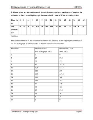
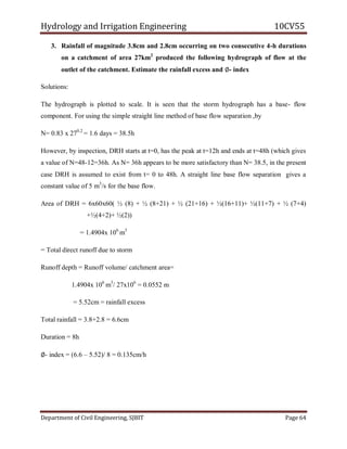
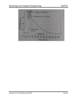
Downloaded 574 times
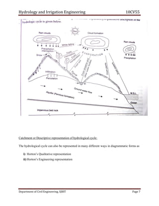
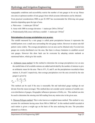
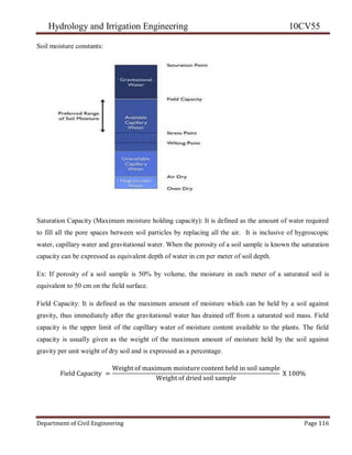
![Hydrology and Irrigation Engineering 10CV55
Department of Civil Engineering, SJBIT Page 83
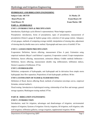
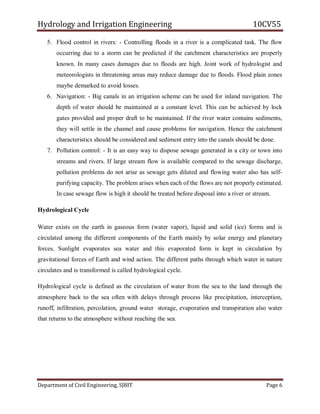
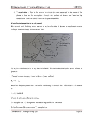
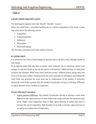
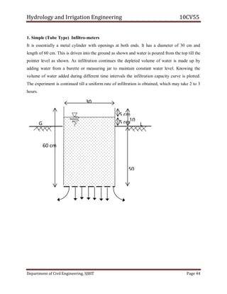
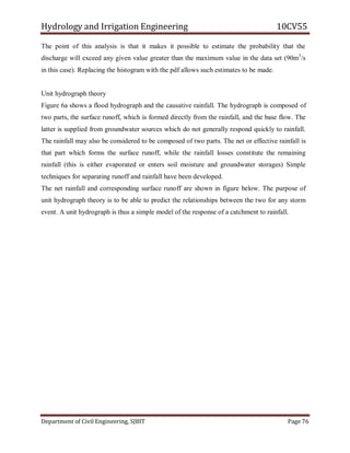
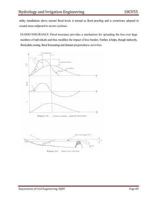
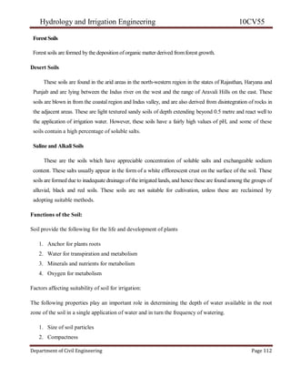
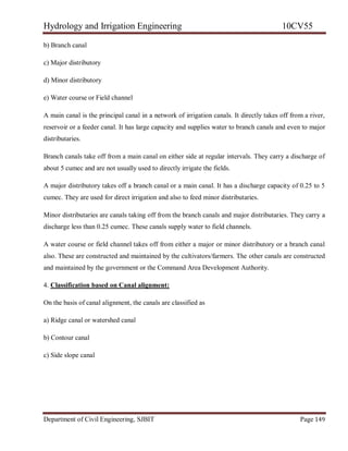
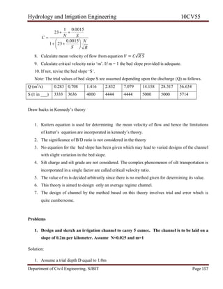
ESTIMATION OF K AND x
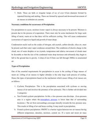
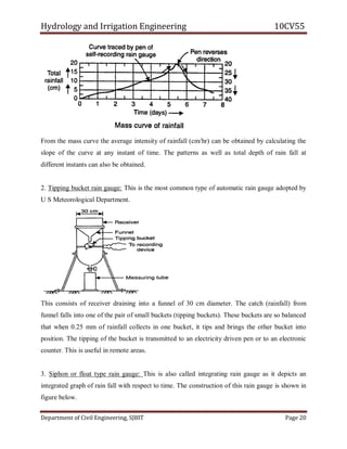
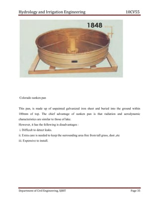
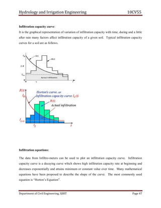
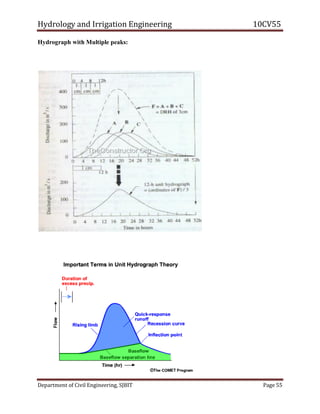
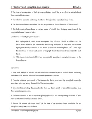
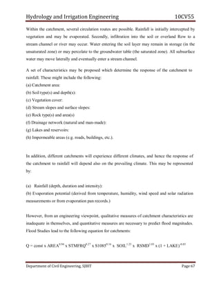
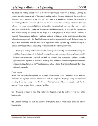
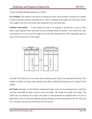
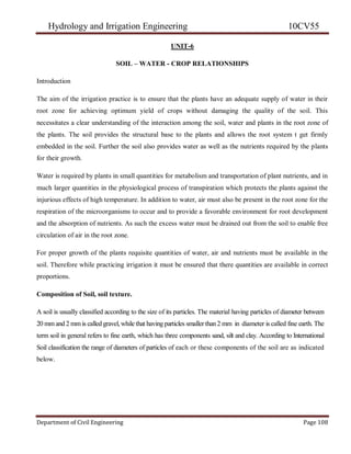
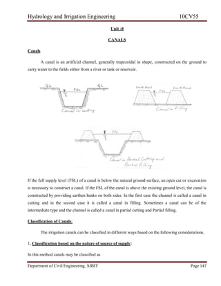
Figure 8.8 shows a typical inflow and
outflow hydrograph through a
channel reach. Note that the outflow
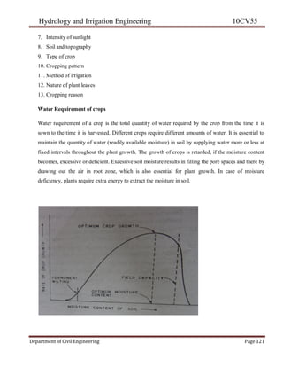
peak does not occur at the point of
intersection of the inflow and outflow
hydrographs. Using the continuity
equation [Eq. (8.3)]
the increment in storage at any time t and
time element At can be calculated. Summation of the
various incremental storage values enables one to find
the channel storage S vs time f relationship (Fig. 8.8).
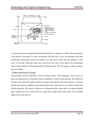
If an inflow and outflow hydrograph set is available
for a given reach, values of S at various time intervals
can be determined by the above technique. By
choosing a trial value of x, values of S at any time t are
plotted against the Time
Corresponding to [x I+ (1 -x) Q] values.
If the value of x is chosen correctly, a straight-line relationship as given by Eq. (8.12) will result
However, if an incorrect value of x is used, the plotted points will trace a looping curve By trial and
value of x is so chosen that the data very nearly describe a straight line (Fig 8.9) inverse slope of
this straight line will give the value of K:
Normally, for natural channels, the value of x lies between 0 to 0 3 For a reach, the values of x
and K are assumed to be constant
Lag
* ----- =-►
Attenuation1](https://image.slidesharecdn.com/civil-v-hydrologyandirrigationengineering10cv55-notes-160425135643/85/Civil-v-hydrology-and-irrigation-engineering-10-cv55-notes-83-320.jpg)
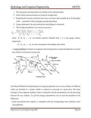
![Hydrology and Irrigation Engineering 10CV55
Department of Civil Engineering, SJBIT Page 142
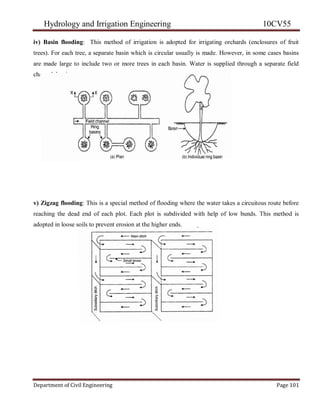
If the frequency of irrigation is 10 days and the overall efficiency is 23%,fina
(i) the daily consumptive use (ii) The water discharge in m2
/sec required in the canal feeding the
area.
Solution
dw = Sg.d [Fc - m0] = 1.4 x 80 [0.26 - 0.12]=15.68 cm
Frequency of irrigation = 10 days.
Daily consumption use= 15.68/10= 1.568cm= 15.68mm
Total water required in 10 days= Ax dw= 3000x 104
x 15.68/100= 4704000m3
Discharge in the canal= 4704000/(10x24x3600) = 5.45 cumecs
Problems 4.
The gross commanded area for a distributory is 20000 hectares,75% of which can be irrigated.
The intensity of irrigation for Rabi season is 40% that for Kharif season is 10%. If kor period is
4 weeks for rabi and 2.5 weeks for rice, determine he outlet discharge . Outlet factors for rabi and
rice may be assumed as 1800 hectares/ cumec and 775 hectares/ cumec. Also calculate delta for each
crop.
Gross commanded area = 20000 hectares
Culturable commanded area = 0.75 x 20000 = 15000 hectares.
Area under irrigation in Rabi season at 40% intensity = 15000 x 0.4 = 6000 hectares
Area under irrigation in Kharif season at 10% intensity = 15000 x 0.1 = 1500 hectares.
Outlet Discharge for Rabi = 6000/1800= 3.33 cumec
Outlet Discharge for Kharif = 1500/775= 1.94cumec
From the equation
Similarly for rabi ∆= 8.64𝐵/𝐷](https://image.slidesharecdn.com/civil-v-hydrologyandirrigationengineering10cv55-notes-160425135643/85/Civil-v-hydrology-and-irrigation-engineering-10-cv55-notes-142-320.jpg)
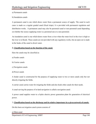

The document outlines the syllabus for a course on Hydrology and Irrigation Engineering, detailing various units covering topics such as the hydrologic cycle, precipitation, evaporation, hydrographs, flood estimation, and irrigation systems. It includes definitions, measurement methods, and the importance of hydrology in civil engineering applications like water supply, irrigation, flood control, and hydroelectric power generation. Additionally, it lists textbooks and reference materials related to the subject.