Download to read offline


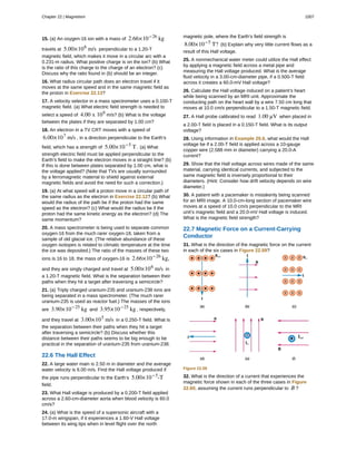


![6. The direction (or polarity) of the induced emf will now drive a current in this direction and can be represented as current
emerging from the positive terminal of the emf and returning to its negative terminal.
For practice, apply these steps to the situations shown in Figure 23.7 and to others that are part of the following text material.
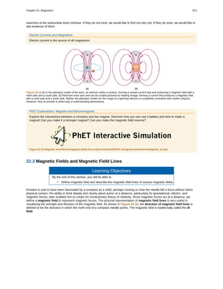
Applications of Electromagnetic Induction
There are many applications of Faraday’s Law of induction, as we will explore in this chapter and others. At this juncture, let us
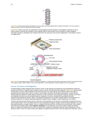
mention several that have to do with data storage and magnetic fields. A very important application has to do with audio and
video recording tapes. A plastic tape, coated with iron oxide, moves past a recording head. This recording head is basically a
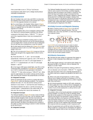
round iron ring about which is wrapped a coil of wire—an electromagnet (Figure 23.8). A signal in the form of a varying input
current from a microphone or camera goes to the recording head. These signals (which are a function of the signal amplitude
and frequency) produce varying magnetic fields at the recording head. As the tape moves past the recording head, the magnetic
field orientations of the iron oxide molecules on the tape are changed thus recording the signal. In the playback mode, the
magnetized tape is run past another head, similar in structure to the recording head. The different magnetic field orientations of
the iron oxide molecules on the tape induces an emf in the coil of wire in the playback head. This signal then is sent to a
loudspeaker or video player.
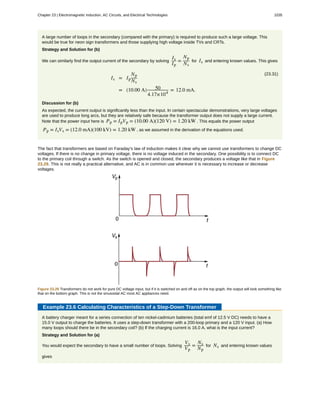
Figure 23.8 Recording and playback heads used with audio and video magnetic tapes. (credit: Steve Jurvetson)
Similar principles apply to computer hard drives, except at a much faster rate. Here recordings are on a coated, spinning disk.
Read heads historically were made to work on the principle of induction. However, the input information is carried in digital rather
than analog form – a series of 0’s or 1’s are written upon the spinning hard drive. Today, most hard drive readout devices do not
work on the principle of induction, but use a technique known as giant magnetoresistance. (The discovery that weak changes in
a magnetic field in a thin film of iron and chromium could bring about much larger changes in electrical resistance was one of the
first large successes of nanotechnology.) Another application of induction is found on the magnetic stripe on the back of your
personal credit card as used at the grocery store or the ATM machine. This works on the same principle as the audio or video
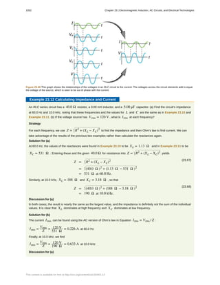
tape mentioned in the last paragraph in which a head reads personal information from your card.
Another application of electromagnetic induction is when electrical signals need to be transmitted across a barrier. Consider the
cochlear implant shown below. Sound is picked up by a microphone on the outside of the skull and is used to set up a varying
magnetic field. A current is induced in a receiver secured in the bone beneath the skin and transmitted to electrodes in the inner
ear. Electromagnetic induction can be used in other instances where electric signals need to be conveyed across various media.
Figure 23.9 Electromagnetic induction used in transmitting electric currents across mediums. The device on the baby’s head induces an electrical
current in a receiver secured in the bone beneath the skin. (credit: Bjorn Knetsch)
Another contemporary area of research in which electromagnetic induction is being successfully implemented (and with
substantial potential) is transcranial magnetic simulation. A host of disorders, including depression and hallucinations can be
traced to irregular localized electrical activity in the brain. In transcranial magnetic stimulation, a rapidly varying and very
localized magnetic field is placed close to certain sites identified in the brain. Weak electric currents are induced in the identified
sites and can result in recovery of electrical functioning in the brain tissue.
Sleep apnea (“the cessation of breath”) affects both adults and infants (especially premature babies and it may be a cause of
sudden infant deaths [SID]). In such individuals, breath can stop repeatedly during their sleep. A cessation of more than 20
seconds can be very dangerous. Stroke, heart failure, and tiredness are just some of the possible consequences for a person
having sleep apnea. The concern in infants is the stopping of breath for these longer times. One type of monitor to alert parents
when a child is not breathing uses electromagnetic induction. A wire wrapped around the infant’s chest has an alternating current
running through it. The expansion and contraction of the infant’s chest as the infant breathes changes the area through the coil.
A pickup coil located nearby has an alternating current induced in it due to the changing magnetic field of the initial wire. If the
child stops breathing, there will be a change in the induced current, and so a parent can be alerted.
1020 Chapter 23 | Electromagnetic Induction, AC Circuits, and Electrical Technologies
This content is available for free at http://cnx.org/content/col11844/1.13](https://image.slidesharecdn.com/ap2unit5openstaxnotes-160229020538/85/Ap2-unit5-open-stax-notes-56-320.jpg)


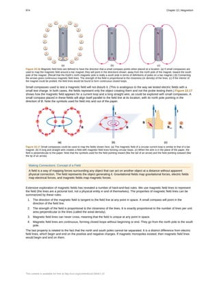
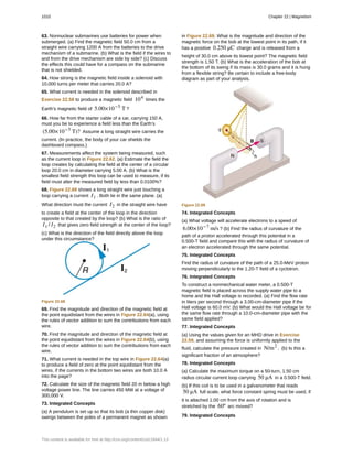
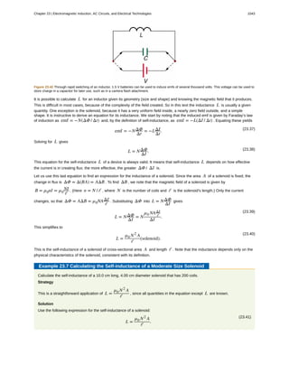
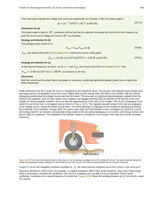
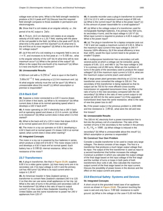
![Figure 23.40 The heating coils of an electric clothes dryer can be counter-wound so that their magnetic fields cancel one another, greatly reducing the
mutual inductance with the case of the dryer.
Self-inductance, the effect of Faraday’s law of induction of a device on itself, also exists. When, for example, current through a
coil is increased, the magnetic field and flux also increase, inducing a counter emf, as required by Lenz’s law. Conversely, if the
current is decreased, an emf is induced that opposes the decrease. Most devices have a fixed geometry, and so the change in
flux is due entirely to the change in current ΔI through the device. The induced emf is related to the physical geometry of the
device and the rate of change of current. It is given by
(23.36)
emf = −LΔI
Δt
,
where L is the self-inductance of the device. A device that exhibits significant self-inductance is called an inductor, and given
the symbol in Figure 23.41.
Figure 23.41
The minus sign is an expression of Lenz’s law, indicating that emf opposes the change in current. Units of self-inductance are
henries (H) just as for mutual inductance. The larger the self-inductance L of a device, the greater its opposition to any change
in current through it. For example, a large coil with many turns and an iron core has a large L and will not allow current to
change quickly. To avoid this effect, a small L must be achieved, such as by counterwinding coils as in Figure 23.40.
A 1 H inductor is a large inductor. To illustrate this, consider a device with L = 1.0 H that has a 10 A current flowing through it.
What happens if we try to shut off the current rapidly, perhaps in only 1.0 ms? An emf, given by emf = −L(ΔI / Δt) , will
oppose the change. Thus an emf will be induced given by emf = −L(ΔI / Δt) = (1.0 H)[(10 A) / (1.0 ms)] = 10,000 V .
The positive sign means this large voltage is in the same direction as the current, opposing its decrease. Such large emfs can
cause arcs, damaging switching equipment, and so it may be necessary to change current more slowly.
There are uses for such a large induced voltage. Camera flashes use a battery, two inductors that function as a transformer, and
a switching system or oscillator to induce large voltages. (Remember that we need a changing magnetic field, brought about by a
changing current, to induce a voltage in another coil.) The oscillator system will do this many times as the battery voltage is
boosted to over one thousand volts. (You may hear the high pitched whine from the transformer as the capacitor is being
charged.) A capacitor stores the high voltage for later use in powering the flash. (See Figure 23.42.)
1042 Chapter 23 | Electromagnetic Induction, AC Circuits, and Electrical Technologies
This content is available for free at http://cnx.org/content/col11844/1.13](https://image.slidesharecdn.com/ap2unit5openstaxnotes-160229020538/85/Ap2-unit5-open-stax-notes-78-320.jpg)


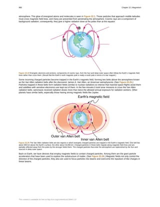
1) Magnets have two poles, a north pole and a south pole. Like poles repel and unlike poles attract. Magnetic poles always occur in pairs and cannot be separated. 2) Ferromagnetic materials contain small magnetic regions called domains that act like magnets. In an external magnetic field, the domains align to strongly magnetize the material. Above the Curie temperature, ferromagnets lose their magnetism. 3) Electromagnets use electric currents to generate magnetic fields and act similarly to permanent magnets. They are widely used in applications requiring strong, controllable magnetic fields.


